Installing Python
This page has been moved to https://econ.pages.code.wm.edu/414/syllabus/docs/index.html and is no longer being maintained here.
This short guide will help you get started with the anaconda python distribution on your PC or MAC. If you happen to run linux, please contact Professor Hicks directly.
Important Note:
Please use a pristine Anaconda Python install for this class. If you have an existing Anaconda install that you would like to keep, please see me about your options. If you have an existing Anaconda install, and don't care to keep it, just delete the folder prior to initiating the installation steps below. Just take care to save any of your work in the Anaconda folder before deleting it.
Installing Python
Both the PC and MAC installers can be downloaded at https://www.anaconda.com/download/. Choose the 64bit Python 3.x version for your platform (3.7 at the time of this writing).
This short guide will help you get started with the anaconda python distribution on your PC or MAC. If you happen to run linux, please contact Professor Hicks directly.
Once you have downloaded the installer, do the following:
- Navigate to your your browser's download folder
- Open the python executable downloaded in step (1) (e.g. Anaconda-3.x.x-Windows-x_86_64.exe [PC] or Anaconda-3.x-mac-x_86_64.dmg [MAC])
- Click through the install screens and choose to install "Just Me" and don't change the default install location. Leave any "Advanced Options" at their default values.
Using Python
Now that python is installed we can use it. There are several ways to run python code, and I will show you a method allowing you to use your web browser as a "front-end" for python.
We will be using the Ipython Notebook (now called Jupyter). The easiest way to open it is to locate and use the Anaconda Launcher. Hopefully, the install process will put this in your Program Files (PC) or Applications (Mac). If you see a new icon labeled Anaconda Launcher, click it and choose jupyter notebook. Sometimes, the install process doesn't create the Anaconda icon. In this case, it is possible to locate it in the Anaconda folder in your local home directory.
In case you can't find the Anaconda icon, you can also launch it from the terminal or command prompt window, type jupyter notebook.
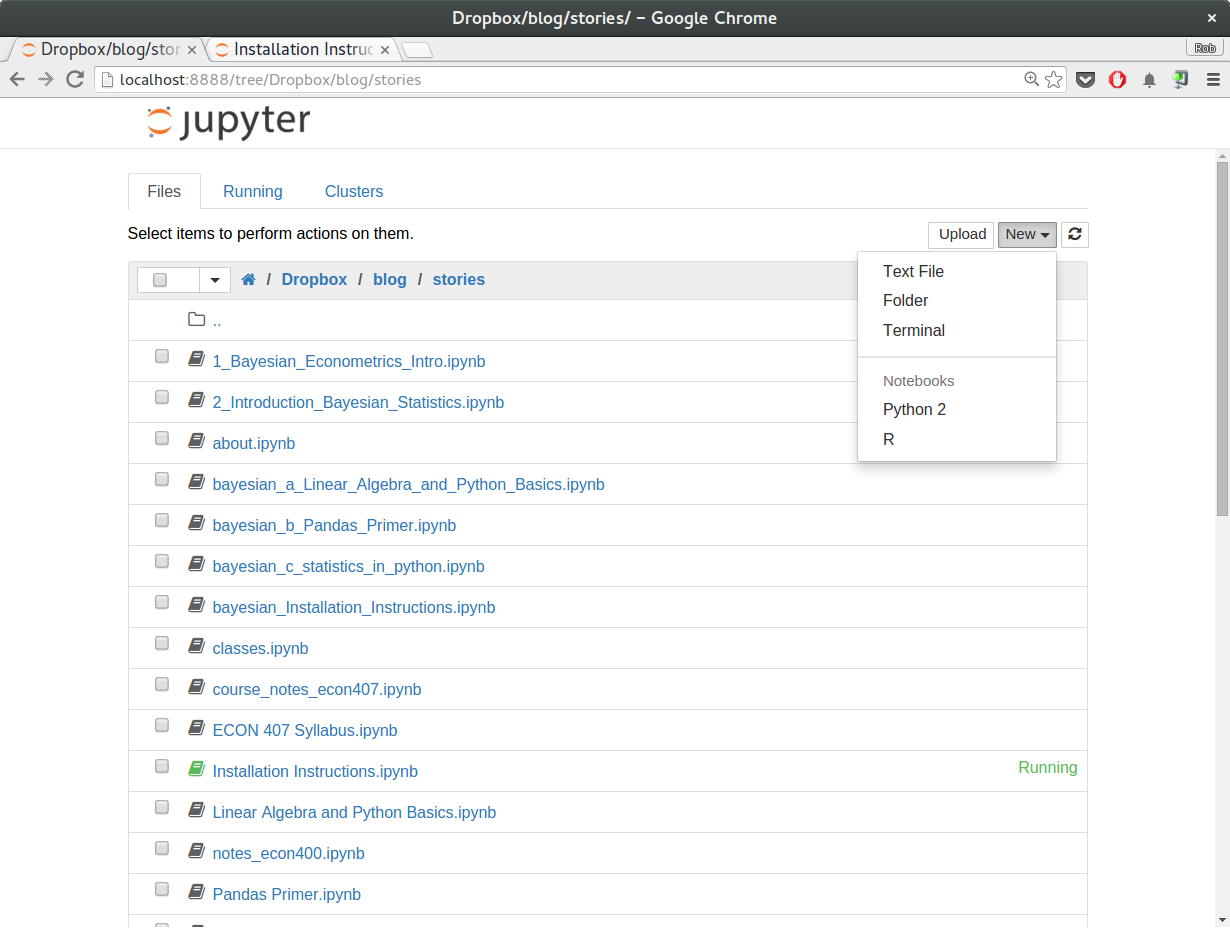
If you have made it this far, your web browser should pop up and you should see a window like this (note: the actual filenames and folders you will see will reflect the actual information you have on your computer):
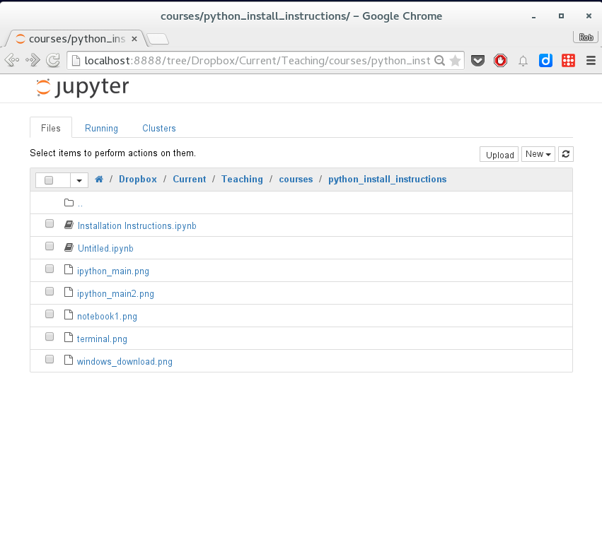
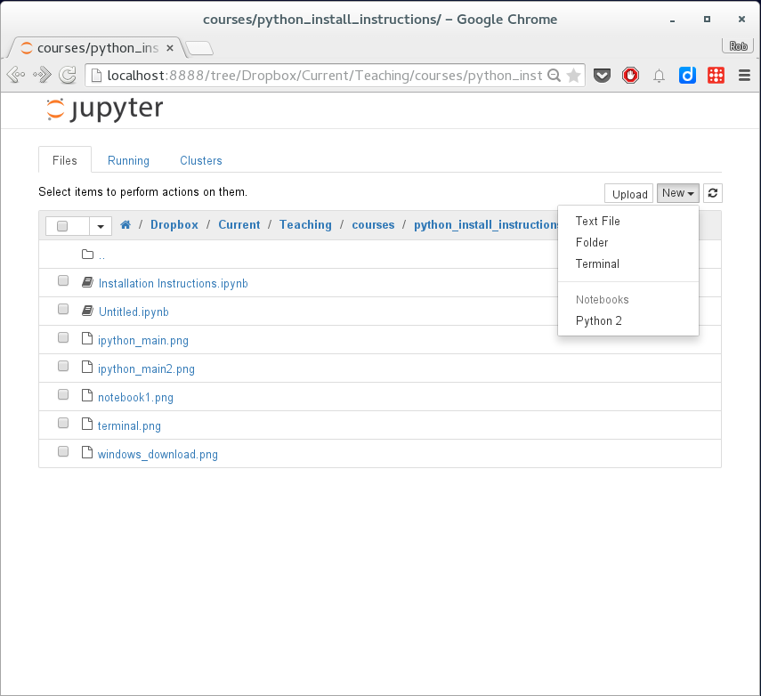
This listing allows you to see existing and running Ipython Notebooks. You won't have any, so let's create one. You can navigate to a folder of your choosing and create a new notebook by clicking on New and then Python 3 as shown below [Note, the screenshot below is from an old python version and shows Python 2):
Testing the installation
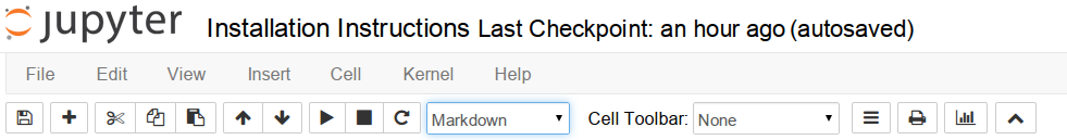
Having created a new notebook, you should see a window that looks like this:
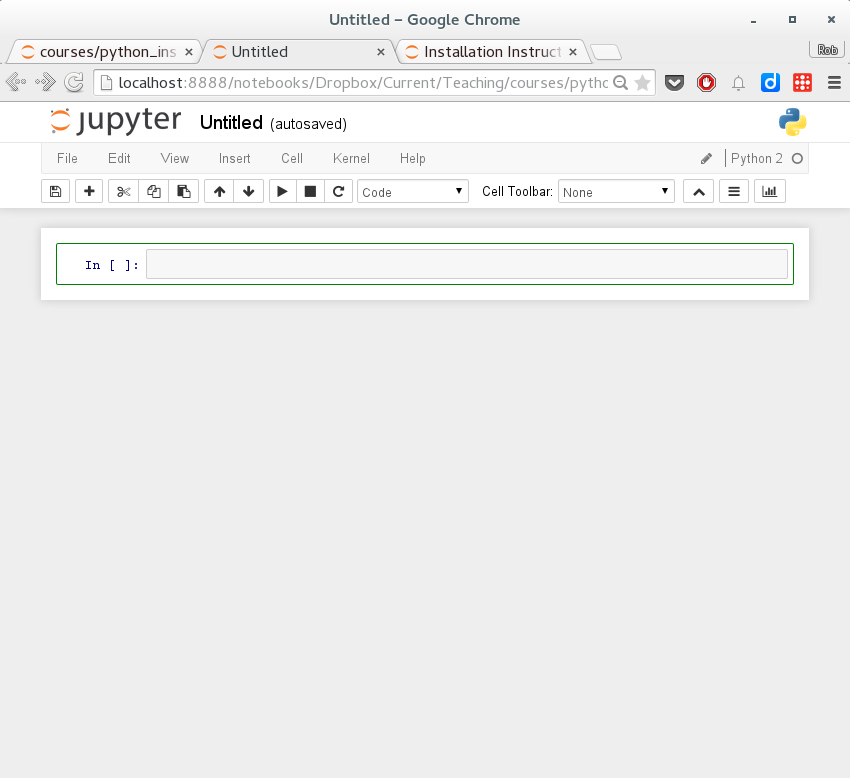
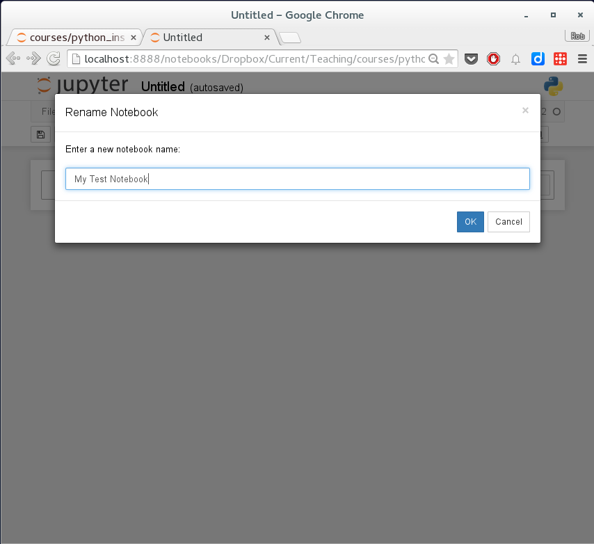
You can re-name your new untitled notebook by clicking on Untitled and changing the name:
Ipython Notebooks have execution blocks where you can enter and execute python code. These blocks look like this:

Copy and paste the following code into the first (and only at this point) execution block:
%matplotlib inline
import pandas as pd
import numpy as np
import matplotlib.pyplot as plt
import statsmodels.formula.api as sm
import sympy as sympy
You should see output like this after pressing the shift enter keys at the same time to execute the code:
%matplotlib inline
import pandas as pd
import numpy as np
import matplotlib.pyplot as plt
import statsmodels.formula.api as sm
import sympy as sympy
Next, we will make sure things are working. Paste this code into the next execution cell and press shift enter:
# create some toy data
time=np.arange(1,101)
price = np.random.normal(10,3,(np.size(time)))

# load into pandas dataframe
df = pd.DataFrame(np.c_[time,price],columns=['time','price'])

# run summary statistics
df.describe()
We can also visualize our data easily using the pandas package:
# plot histogram of price
df.price.plot(kind='hist')

# or a trace plot through time:
df.price.plot()

Next we will test the statsmodels library:
import statsmodels.formula.api as smf
formula = "price ~ time"
results = smf.ols(formula,df).fit()
print(results.summary())
Markdown Text and Notebook Annotations
Changing the execution cell type to markdown here:
allows you to enter markdown compliant passages and get nicely formatted text when you execute the cell by pressing shift enter. For example, executing the following markdown code in a markdown execution cell:
This is some markdown code. I can type sentences and paragraphs here. Or, if I want a numbered list, here it is:
1. Dogs
2. Cats
3. Elephants
I can include links in my markdown passages:

And I can include latex equations inline: $\frac{\alpha}{\beta}$. Or I can put them on their own line
$$
W_j = \sum_{i\ne j} W_{ij} \epsilon_i
$$
results in this output:
This is some markdown code. I can type sentences and paragraphs here. Or, if I want a numbered list, here it is:
- Dogs
- Cats
- Elephants
I can include links in my markdown passages:

And I can include latex equations inline: $\frac{\alpha}{\beta}$. Or I can put them on their own line $$ W_j = \sum_{i\ne j} W_{ij} \epsilon_i $$
Youtube Videos
from IPython.display import YouTubeVideo
YouTubeVideo("d0nERTFo-Sk")
Installing Additional Packages
Anaconda has many, but not all, packages we might use. For example, seaborn isn't included. To install it (and other python packages you want that aren't packaged with Anaconda), follow these steps:
Mac or Linux
From inside the ipython notebook desribed above, choose Terminal from the New dropdown box shown below:
You should see a terminal screen that looks something like this:
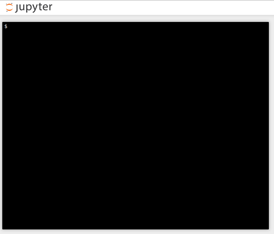
In the terminal prompt, type
conda install seaborn
press enter and after a little time, it should install without incident.
Windows
In Windows, choose Program Files -> Anaconda2 (64-bit) and you should see the following list of programs:
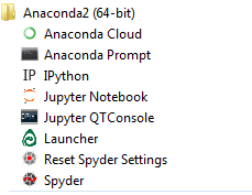
Choose Anaconda Prompt and at the command prompt, type
conda install seaborn
press enter and after a little time, it should install without incident.
Installing pymc3
The best way to install packages is via the conda command.
conda install pymc3
The required compiler packages and other necessities should automatically be installed so that pymc3 models will compile and run as required for this class.