Comparing Stata and Ipython Commands for OLS Models
In this note, I’ll explore the Ipython statsmodels package for estimating linear regression models (OLS). The goal is to completely map stata commands for reg into something implementable in Ipython.
#load python libraries for this ipython notebook:
%matplotlib inline
import pandas as pd             # pandas data manipulation library
import statsmodels.formula.api as smf    # for the ols and robust ols model
import statsmodels.api as sm
import numpy as np
Note this is from the Tobias and Koop dataset on the returns to education. The full dataset is a panel. I have turned this into a cross section where time==4 (for demonstration purposes only).
# load data and create dataframe
tobias_koop=pd.read_csv('http://rlhick.people.wm.edu/econ407/data/tobias_koop_t_4.csv')
With the pandas data frame created, we can easily run some models. First let’s look at the data, run summary statistics, and plot the histogram of our dependent variable, ln_wage.
tobias_koop.head()| id | educ | ln_wage | pexp | time | ability | meduc | feduc | broken_home | siblings | pexp2 | |
|---|---|---|---|---|---|---|---|---|---|---|---|
| 0 | 4 | 12 | 2.14 | 2 | 4 | 0.26 | 12 | 10 | 1 | 4 | 4 |
| 1 | 6 | 15 | 1.91 | 4 | 4 | 0.44 | 12 | 16 | 0 | 2 | 16 |
| 2 | 8 | 13 | 2.32 | 8 | 4 | 0.51 | 12 | 15 | 1 | 2 | 64 |
| 3 | 11 | 14 | 1.64 | 1 | 4 | 1.82 | 16 | 17 | 1 | 2 | 1 |
| 4 | 12 | 13 | 2.16 | 6 | 4 | -1.30 | 13 | 12 | 0 | 5 | 36 |
tobias_koop.describe()| id | educ | ln_wage | pexp | time | ability | meduc | feduc | broken_home | siblings | pexp2 | |
|---|---|---|---|---|---|---|---|---|---|---|---|
| count | 1034.000000 | 1034.000000 | 1034.000000 | 1034.000000 | 1034 | 1034.000000 | 1034.000000 | 1034.000000 | 1034.000000 | 1034.000000 | 1034.000000 |
| mean | 1090.951644 | 12.274662 | 2.138259 | 4.815280 | 4 | 0.016596 | 11.403288 | 11.585106 | 0.169246 | 3.200193 | 27.979691 |
| std | 634.891728 | 1.566838 | 0.466280 | 2.190298 | 0 | 0.920963 | 3.027277 | 3.735833 | 0.375150 | 2.126575 | 22.598790 |
| min | 4.000000 | 9.000000 | 0.420000 | 0.000000 | 4 | -3.140000 | 0.000000 | 0.000000 | 0.000000 | 0.000000 | 0.000000 |
| 25% | 537.250000 | 12.000000 | 1.820000 | 3.000000 | 4 | -0.550000 | 11.000000 | 10.000000 | 0.000000 | 2.000000 | 9.000000 |
| 50% | 1081.500000 | 12.000000 | 2.120000 | 5.000000 | 4 | 0.170000 | 12.000000 | 12.000000 | 0.000000 | 3.000000 | 25.000000 |
| 75% | 1666.500000 | 13.000000 | 2.450000 | 6.000000 | 4 | 0.720000 | 12.000000 | 14.000000 | 0.000000 | 4.000000 | 36.000000 |
| max | 2177.000000 | 19.000000 | 3.590000 | 12.000000 | 4 | 1.890000 | 20.000000 | 20.000000 | 1.000000 | 15.000000 | 144.000000 |
tobias_koop.ln_wage.plot(kind='hist')<matplotlib.axes.AxesSubplot at 0x41dcb50>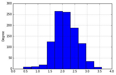
OLS analysis
This is the model we’ll be estimating the vector \(\) from
\[ y_i = \beta_0 + \beta_1 educ_i + \beta_2 pexp_i + \beta_3 pexp^2_i + \beta_4 broken\_home_i + \epsilon_i \]
For now, we will ignore any potential bias due to endogeneity, although we’ll come back to that in a later post.
Fitting the model in stata
Here is the code for estimating the model in stata:
. reg ln_wage educ pexp pexp2 broken_home

      Source |       SS       df       MS              Number of obs =    1034
-------------+------------------------------           F(  4,  1029) =   51.36
       Model |  37.3778146     4  9.34445366           Prob > F      =  0.0000
    Residual |   187.21445  1029  .181938241           R-squared     =  0.1664
-------------+------------------------------           Adj R-squared =  0.1632
       Total |  224.592265  1033  .217417488           Root MSE      =  .42654

------------------------------------------------------------------------------
     ln_wage |      Coef.   Std. Err.      t    P>|t|     [95% Conf. Interval]
-------------+----------------------------------------------------------------
        educ |   .0852725   .0092897     9.18   0.000     .0670437    .1035014
        pexp |   .2035214   .0235859     8.63   0.000     .1572395    .2498033
       pexp2 |  -.0124126   .0022825    -5.44   0.000    -.0168916   -.0079336
 broken_home |  -.0087254   .0357107    -0.24   0.807    -.0787995    .0613488
       _cons |   .4603326    .137294     3.35   0.001     .1909243    .7297408
------------------------------------------------------------------------------
Fitting the model Ipython with statsmodels
We will estimate the same models as above using statsmodels.
formula = "ln_wage ~ educ + pexp + pexp2 + broken_home"
results = smf.ols(formula,tobias_koop).fit()
print(results.summary())
OLS Regression Results
==============================================================================
Dep. Variable: ln_wage R-squared: 0.166
Model: OLS Adj. R-squared: 0.163
Method: Least Squares F-statistic: 51.36
Date: Thu, 05 Mar 2015 Prob (F-statistic): 1.83e-39
Time: 09:18:38 Log-Likelihood: -583.66
No. Observations: 1034 AIC: 1177.
Df Residuals: 1029 BIC: 1202.
Df Model: 4
Covariance Type: nonrobust
===============================================================================
coef std err t P>|t| [95.0% Conf. Int.]
-------------------------------------------------------------------------------
Intercept 0.4603 0.137 3.353 0.001 0.191 0.730
educ 0.0853 0.009 9.179 0.000 0.067 0.104
pexp 0.2035 0.024 8.629 0.000 0.157 0.250
pexp2 -0.0124 0.002 -5.438 0.000 -0.017 -0.008
broken_home -0.0087 0.036 -0.244 0.807 -0.079 0.061
==============================================================================
Omnibus: 55.892 Durbin-Watson: 1.761
Prob(Omnibus): 0.000 Jarque-Bera (JB): 112.050
Skew: -0.355 Prob(JB): 4.66e-25
Kurtosis: 4.448 Cond. No. 391.
==============================================================================
Warnings:
[1] Standard Errors assume that the covariance matrix of the errors is correctly specified.OLS Regression with robust standard errors
Recall that for robust standard errors, we first recover our OLS estimates (\(\mathbf{b}\)) of \(\beta\). Using \(\mathbf{b}\), construct \(\mathbf{e} = \mathbf{y - xb}\). From there, calculate the robust variance/covariance matrix of estimated parameters as \[ Var(\mathbf{b})_{robust} = \mathbf{(x'x)^{-1}x'diag(ee')x(x'x)^{-1}}\times \frac{N}{N-K} \] for calculating standard errors.
Fitting the model in stata
In stata, we would run this:
. reg ln_wage educ pexp pexp2 broken_home, robust

Linear regression                                      Number of obs =    1034
                                                       F(  4,  1029) =   64.82
                                                       Prob > F      =  0.0000
                                                       R-squared     =  0.1664
                                                       Root MSE      =  .42654

------------------------------------------------------------------------------
             |               Robust
     ln_wage |      Coef.   Std. Err.      t    P>|t|     [95% Conf. Interval]
-------------+----------------------------------------------------------------
        educ |   .0852725   .0099294     8.59   0.000     .0657882    .1047568
        pexp |   .2035214   .0226835     8.97   0.000     .1590101    .2480326
       pexp2 |  -.0124126   .0022447    -5.53   0.000    -.0168173   -.0080079
 broken_home |  -.0087254   .0312381    -0.28   0.780     -.070023    .0525723
       _cons |   .4603326   .1315416     3.50   0.000     .2022121     .718453
------------------------------------------------------------------------------
Fitting the model in Ipython
In Ipython, we don’t need to rerun the model. The default OLS command already includes a number of different types of robust standard errors (one of which using the method outlined above). All we need to do is create a new results instance that calls the covariance type we want:
results_robust = results.get_robustcov_results(cov_type='HC1')
print(results_robust.summary())
OLS Regression Results
==============================================================================
Dep. Variable: ln_wage R-squared: 0.166
Model: OLS Adj. R-squared: 0.163
Method: Least Squares F-statistic: 64.82
Date: Thu, 05 Mar 2015 Prob (F-statistic): 6.41e-49
Time: 09:18:39 Log-Likelihood: -583.66
No. Observations: 1034 AIC: 1177.
Df Residuals: 1029 BIC: 1202.
Df Model: 4
Covariance Type: HC1
===============================================================================
coef std err t P>|t| [95.0% Conf. Int.]
-------------------------------------------------------------------------------
Intercept 0.4603 0.132 3.500 0.000 0.202 0.718
educ 0.0853 0.010 8.588 0.000 0.066 0.105
pexp 0.2035 0.023 8.972 0.000 0.159 0.248
pexp2 -0.0124 0.002 -5.530 0.000 -0.017 -0.008
broken_home -0.0087 0.031 -0.279 0.780 -0.070 0.053
==============================================================================
Omnibus: 55.892 Durbin-Watson: 1.761
Prob(Omnibus): 0.000 Jarque-Bera (JB): 112.050
Skew: -0.355 Prob(JB): 4.66e-25
Kurtosis: 4.448 Cond. No. 391.
==============================================================================
Warnings:
[1] Standard Errors are heteroscedasticity robust (HC1)Bootstrapped standard errors
Fitting the model in stata
If instead, we want to bootstrap our standard errors, in stata we would do this:
. bstrap:  reg ln_wage educ pexp pexp2 broken_home
(running regress on estimation sample)

Bootstrap replications (50)
----+--- 1 ---+--- 2 ---+--- 3 ---+--- 4 ---+--- 5
..................................................    50

Linear regression                               Number of obs      =      1034
                                                Replications       =        50
                                                Wald chi2(4)       =    290.46
                                                Prob > chi2        =    0.0000
                                                R-squared          =    0.1664
                                                Adj R-squared      =    0.1632
                                                Root MSE           =    0.4265

------------------------------------------------------------------------------
             |   Observed   Bootstrap                         Normal-based
     ln_wage |      Coef.   Std. Err.      z    P>|z|     [95% Conf. Interval]
-------------+----------------------------------------------------------------
        educ |   .0852725    .010622     8.03   0.000     .0644539    .1060912
        pexp |   .2035214   .0217148     9.37   0.000     .1609611    .2460816
       pexp2 |  -.0124126   .0021076    -5.89   0.000    -.0165433   -.0082818
 broken_home |  -.0087254   .0330727    -0.26   0.792    -.0735466    .0560958
       _cons |   .4603326   .1405716     3.27   0.001     .1848173    .7358479
------------------------------------------------------------------------------
It is important to note that the above set of results implicitly assumes normality, since confidence intervals are symmetric about the mean (and since standard errors are reported).
Fitting the model in Ipython
This isn’t as straightforward in Ipython. We need to do a bit of wrangling to get the bootstrap working in Ipython. Write our own routine.
R = 50

results_boot = np.zeros((R,results.params.shape[0]))

row_id = range(0,tobias_koop.shape[0])

for r in range(R):
     this_sample = np.random.choice(row_id, size=tobias_koop.shape[0], replace=True) # gives sampled row numbers
     # Define data for this replicate:
     tobias_koop_r = tobias_koop.iloc[this_sample]
     # Estimate model
     results_r = smf.ols(formula,tobias_koop_r).fit(disp=0).params
     # Store in row r of results_boot:
     results_boot[r,:] = np.asarray(results_r)
The array results_boot has all of our data. Put in pandas dataframe and summarize:
# Convert results to pandas dataframe for easier analysis:
results_boot = pd.DataFrame(results_boot,columns=['b_Intercept','b_educ','b_pexp','pexp2','b_broken_home'])
results_boot.describe(percentiles=[.025,.975])| b_Intercept | b_educ | b_pexp | pexp2 | b_broken_home | |
|---|---|---|---|---|---|
| count | 50.000000 | 50.000000 | 50.000000 | 50.000000 | 50.000000 |
| mean | 0.462494 | 0.084486 | 0.208471 | -0.012965 | -0.017659 |
| std | 0.160763 | 0.011046 | 0.024721 | 0.002473 | 0.036356 |
| min | 0.004603 | 0.056518 | 0.148656 | -0.019397 | -0.102527 |
| 2.5% | 0.126781 | 0.064798 | 0.157471 | -0.018137 | -0.100246 |
| 50% | 0.462583 | 0.084843 | 0.209224 | -0.013365 | -0.010556 |
| 97.5% | 0.783207 | 0.105074 | 0.260848 | -0.008159 | 0.054402 |
| max | 0.801684 | 0.118317 | 0.273543 | -0.007170 | 0.066333 |
In the above set of results, the standard deviation (std) can be interpreted as the parameter standard error if we are willing to impose normality. Alternatively, we could construct 95% confidence intervals by looking at the 2.5% and 97.5% percentiles.