Introduction to Panel Data¶

In this chapter we’ll discuss how to implement a model that relaxes some of the restrictions inherent in the OLS model for cases where you have panel data. To formalize what we mean by panel data, consider a sample of \(N\) individuals, who are each observed in one of \(T\) time periods 1. The model we consider here allows for partial parameter heterogeneity, that is an unobservable individual-specific bit of information varies from individual to individual.

Consider the following figure outlining the effect of possible bias resulting from using a simple OLS model in cases like this. We might ignore any heterogeneity in the relationship (assuming in a pooled model that all \(\beta\)’s are the same across the three individuals) and estimate a relationship like the one depicted in the figure and labeled ‘OLS Estimate’. Note that this model restricts \(c_i=c\) \(\forall i\in N\). The true relationship, however, as depicted by the colored lines, may exhibit parameter heterogeneity (note that the constant term for each of the dotted lines is different) across groups, while the slope coefficient is the same across the three groups 2. Note that not only do we recover the wrong constant terms using OLS, we also have an estimated regression line that has the wrong sign compared to the “true” relationship.

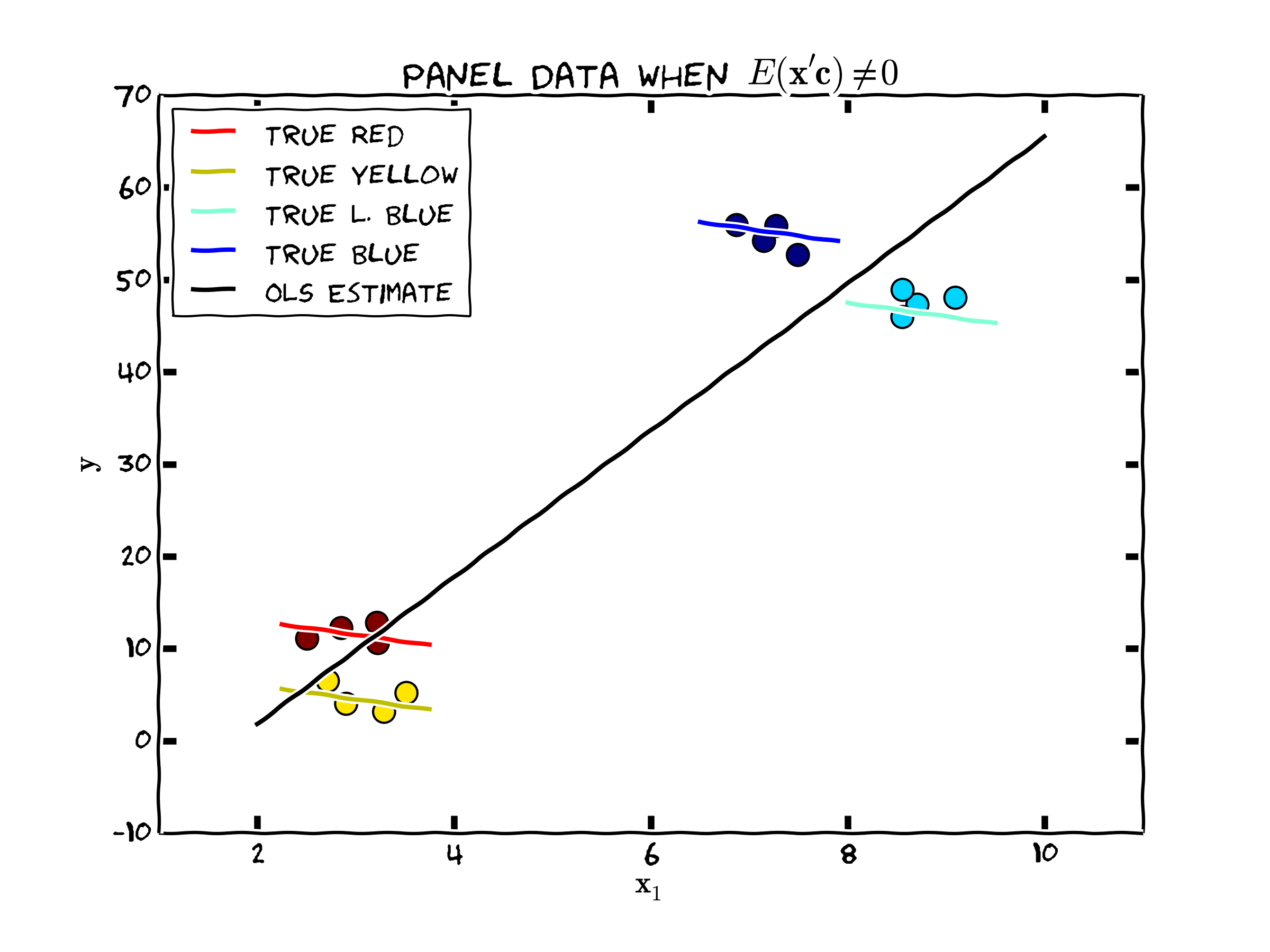
Fig. 3 Bias if we ignore individual heterogeneity¶

However, there may be cases, where ordinary least squares doesn’t fare as poorly and yields consistent estimates for \(\beta\). The following figure shows such a case (that as we will see is suitable for the Random Effects Model).

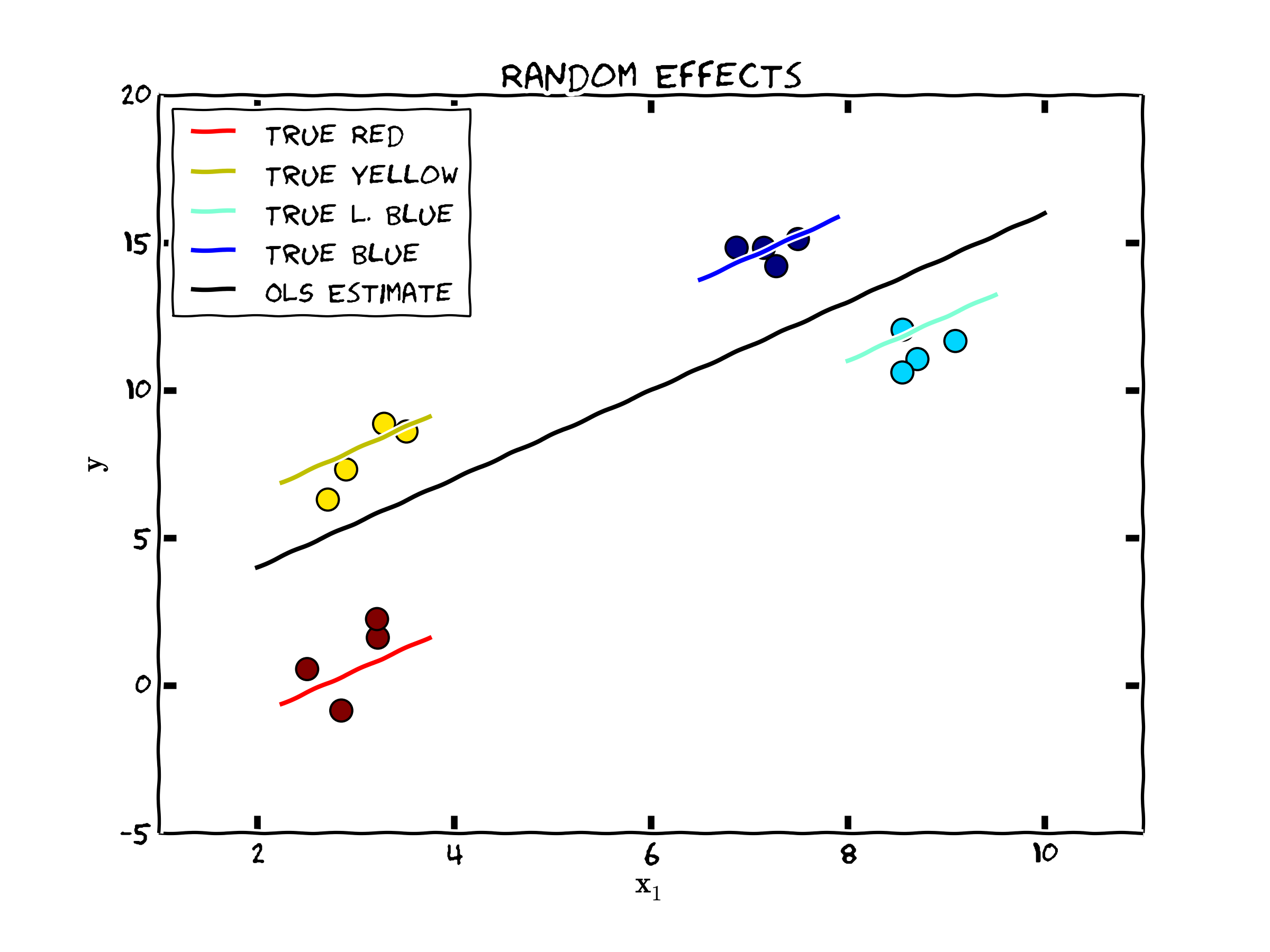
Fig. 4 Sometimes we can ignore individual heterogeneity¶

Framework for Panel Data¶

To formalize this, consider a model of the dependent variable \(y\) that is a linear function of \(K\) independent variables (and parameters) and an individual specific unobservable factors \(c_i\). Write this as

\[\begin{equation} y_{it}=x_{it}\beta+c_i+\epsilon_{it} \end{equation}\]

where \(\beta\) is of dimension \(K\times 1\). If \(c_i\) is uncorrelated with each \(x_{it}\) then we can proceed using OLS and allow the effect of \(c_i\) to be soaked up into the error term. If on the other hand \(c_i\) is correlated with \(x_{it}\) (\(cov(x_i,c_i) \ne 0\)), then putting the effect of \(c_i\) in the error term can lead to biased estimated of \(\beta\) by way of missing variable bias.

Note that we are assuming that the unobserved individual specific effects (\(c_i\)) are constant across time. What is the economic meaning of \(c_i\)? If we are estimating the labor market decisions of women in their twenties and we observed these women in each year, then this time invariant unobservable information might be capturing cognitive ability, drive and determination, or family upbringing that may well influence outcomes for an individual but not vary over time. If our unit of analysis is a firm in an analysis of productivity, \(c_i\) might be capturing information about the managerial ability or organization that is roughly constant through time. Ultimately, these unobserved factors are not of direct interest in these models, we need to worry about them to avoid biased parameters of the marginal effects

\[\begin{equation} \beta=\frac{\partial E[y_{it}|x_{it}]}{\partial x_{it}} \end{equation}\]

To estimate these marginal effects, we need to invoke some assumptions. As in the OLS case, we need exogeneity

\[\begin{equation} E(\epsilon_{t}|\mathbf{x}_{t},\mathbf{c})=0 \end{equation}\]

Which gives us the familiar condition that

(11)¶\[\begin{equation} E(\mathbf{x}_{t}'\epsilon_{t})=0 \end{equation}\]

for \(t=1,2\). If we assume that \(E(\mathbf{x}_{t}'c)=0\) then we could pool the data and estimate an OLS model. If this condition does not hold, however, an OLS model will lead to biased and inconsistent parameter estimates.

A Two Period Example of First Differencing¶

Suppose that for each individual, we have a panel of two periods (\(t=1,2\)). Perhaps we could apply a differencing approach for each individual i to rid the model of \(c_i\), since

\[\begin{split}\begin{aligned} \Delta y_{i} = & \beta \left (x_{i2}-x_{i1} \right ) + \left (c_i-c_i \right) + \left (\epsilon_{i2}-\epsilon_{i1} \right) \\ = & \Delta x_{i} \beta + \Delta \epsilon_{i} \end{aligned}\end{split}\]

since the individual-specific effect is time invariant, these constants drop from the model, and we are still left with our parameters of interest (\(\beta\)). So in a panel with two time periods, we are left with one standard cross section equation consisting of individual level data denoted by

\[\Delta y = \Delta x \beta + \Delta \epsilon\]

where

\[\begin{split} \Delta y = \begin{bmatrix} \Delta y_1 \\ \vdots \\ \Delta y_i \\ \vdots \\ \Delta y_N \end{bmatrix} \end{split}\]

and \(\Delta x\) is defined in a similar fashion. Will a simple OLS estimate of this cross section be unbiased and consistent?

The orthogonality condition is the first place to start with answering this question. Recall that in a standard regression model of the previous chapter, the proof of unbiasedness rests with (11), and invoking the fact that \(E(x'\epsilon)=0\) allows us to show that \(E(b)=\beta\). For OLS to be unbiased, we need a similar condition here. Note that this means

(12)¶\[\begin{equation} E(\Delta x' \Delta \epsilon)=0 \end{equation}\]

and the following inverse must exist

(13)¶\[\begin{equation} (\Delta x' \Delta x)^{-1} \end{equation}\]

requiring that \(\Delta x\) must be of full rank.

What are the implications of these assumptions? First consider (12). This condition can be rewritten as

\[\begin{split}\begin{aligned} & E \left [(x_{2}-x_{1})'(\epsilon_{2}-\epsilon_{1}) \right]=0 \\ & E \left [(x_{2}'\epsilon_{2}+x_{1}'\epsilon_{1}-x_{1}'\epsilon_{2}-x_{2}'\epsilon_{1}) \right]=0 \end{aligned}\end{split}\]

The first two terms are zero by definition given assumption (11). Note however, that in this framework, we also need to assume

\[\begin{split}\begin{aligned} E(x_{1}'\epsilon_{2})&=0 \\ E(x_{2}'\epsilon_{1})&=0 \end{aligned}\end{split}\]

these highlight the even more restrictive orthogonality conditions we need to assume to implement this type of approach.

It is also useful to think carefully about (13). Since the matrix \(\Delta x\) is comprised of elements differenced across two periods, x may not contain any variable that is constant across time for every person in the sample. For example, if the Kth element of x were to contain a dummy variable equal 1 if a person’s sex is female and 0 if male, then

\[\begin{split} \Delta x_K= \begin{bmatrix} \color{blue}{1-1} \\ \color{blue}{\vdots} \\ \color{blue}{1-1} \\ \vdots \\ \color{red}{0-0} \\ \color{red}{\vdots} \\ \color{red}{0-0} \\ \vdots \\ \color{green}{1-1} \\ \color{green}{\vdots} \\ \color{green}{1-1} \\ \end{bmatrix} \end{split}\]

so the matrix \(\Delta x\) would not be of full rank since every element in column K is equal to zero. For some of the panel data models we will consider (i.e. the Fixed Effects Model), your independent variables must vary across periods in your panel. This is very important to remember.

Random or Fixed Effects¶

Following from our framework above, the unobserved effects model can be written

\[ y_{it}=x_{it}\beta+c_i+\epsilon_{it} \]

where \(x_{it}\) is \(1 \times K\). The literature has implemented this type of model in a number of ways, but the most prevalent are termed (1) random effects and (2) fixed effects. These terms refer to assumptions about the individual-specific constant terms \(c_i\).

The labels fixed and random effects are misleading. What matters here is the nature of the unobserved, time invariant, and individual-specific quantities. If there is a dependence between these unobserved factors and the observed independent variables we employ the fixed effects approach. If on the other hand, these effects are independent of the observed independent variables, then we use the random effects estimator. We will explore the difference in the models, compare these approaches to Pooled OLS, and develop some test statistics for model selection.

The Pooled OLS Model¶

The pooled model simply applies an OLS estimate to the pooled data set (where each individual i’s data is ordered from \(t=1,\ldots,T\), and then vertically stacked.). For a data set of N individuals across T periods, the vector \(y\) and the matrix \(x\) will look like

\[\begin{split} y=\begin{bmatrix} \color{blue}{y_{11}} \\ \color{blue}{\vdots} \\ \color{blue}{y_{1T}} \\ \vdots \\ \color{red}{y_{i1}} \\ \color{red}{\vdots} \\ \color{red}{y_{iT}} \\ \vdots \\ \color{green}{y_{N1}} \\ \color{green}{\vdots} \\ \color{green}{y_{NT}} \\ \end{bmatrix} x=\begin{bmatrix} \color{blue}{x_{111} \ldots x_{11k} \ldots x_{11K}}\\ \color{blue}{\ddots} \\ \color{blue}{x_{1T} \ldots x_{1T} \ldots x_{1T}}\\ \vdots \\ \color{red}{x_{i1} \ldots x_{i1} \ldots x_{i1}}\\ \color{red}{\ddots} \\ \color{red}{x_{iT} \ldots x_{iT} \ldots x_{iT}}\\ \vdots \\ \color{green}{x_{N1} \ldots x_{N1} \ldots x_{N1}}\\ \color{green}{\ddots} \\ \color{green}{x_{NT} \ldots x_{NT} \ldots x_{NT}} \\ \end{bmatrix} \end{split}\]

For pooled OLS to be the appropriate estimator, we need to assume

Assumption 1: Strict Endogeneity

\[E[\epsilon_{it}|x_{i1},\ldots,x_{iT}]=0\]

Assumption 2: Uncorrelated individual-specific effects

\[E[c_i|x_{i1},\ldots,x_{iT}]=0\]

Defining \(v_{it}=c_i+\epsilon_{it}\) now completely uncorrelated with the covariates, we have an error structure with orthogonality just as in the previous chapter and our analysis of the OLS model. So we can recover the parameter using

\[\mathbf{b_{ols}}=\mathbf{(x'x)}^{-1}\mathbf{x'y}\]

The usual estimate for the variance covariance matrix, and associated standard errors is

\[Var[\mathbf{b_{ols}}]=\mathbf{\sigma^2E_x[(x'x)^{-1}]}\]

Taking note of the error structure inherent in an OLS model (where \(\epsilon_{i}\sim N(0,\sigma I)\)) compared to this case where the error contain the usual \(\epsilon_{it}\sim N(0,\sigma)\) plus \(c_i\) which is shared by each cross section unit (e.g. each individual or firm). This may well introduce a systematic relationship between the composite error (\(v_{it}\)) among cross section units that the OLS variance-covariance estimate ignores. To fix, this can apply the robust standard errors using the technique we discussed in the previous chapter.

Following the recovery of \(\mathbf{b_{ols}}\), calculate the estimated residuals

\[\mathbf{\hat{v}=y-x b_{ols}}\]

Using the notation adopted in the OLS Chapter for correcting for heteroskedasticity, the expected variance-covariance matrix for the error is

\[\label{eq:het_correction_pooled_OLS} E[var(\mathbf{vv'})]=\hat{\mathbf{V}}=diagonal\left(\hat{\mathbf{v}}\hat{\mathbf{v}}' \right )_{N \times N}\]

let’s us write the robust pooled variance covariance matrix of the parameters as

\[Var^{robust}=\mathbf{(x'x)^{-1}(x'\hat{V}x)(x'x)^{-1}}\]

Notice that this equation is exactly equivalent to the definition of robust standard errors in OLS and highlites the strong assumptions we are making when we estimate panel data with a pooled OLS model.

Implementation in R and Stata¶

The companion chapter shows how to implement many of these ideas in R and Stata.

1: In this chapter we will be assuming balanced panels- that is each individual is assumed for each of the \(T\) time periods. Unbalanced panels, where each individual is observed for \(T_i\) periods, where \(T_i \le T\), are also possible and are implemented in most cases seamlessly in Stata. While the mechanics of unbalanced panels are trivial extensions of what we do here, the potential selection bias associated with individuals joining and dropping in and out of a panel data set should be thought about very seriously.
2: It is also possible that rather than partial parameter heterogeneity all parameters differ across individuals- both constant terms and slope coefficients. We do not consider this case in this chapter, but will briefly discuss it in the advanced topics chapter. This model is the one referred to by Greene [Gre07] on page 183 as Model 4, Random Parameters.