Ordinary Least Squares
Consider the population regression equation for a individual \(i\)
where the dependent variable, \(y_i\) is a function of three types of information:
The independent variables \(x_{i1}\), \(x_{i2}\), and \(x_{i3}\)
Behavioral coefficients: \(\beta_0\), \(\beta_1\), \(\beta_2\), and \(\beta_3\)
Disturbance terms: the \(\epsilon_i\)’s in the equation above.
This regression equation seeks to explain how the dependent variable, \(y_i\) varies with the independent variables \(x_1\), \(x_2\), and \(x_3\). Since we as econometric analysts can not hope to observe everything possibly affecting \(y_i\), we also include disturbance terms (\(\epsilon_i\)) that express how individual observations deviate from the structural relationship between the dependent and independent variables.
Matrix and Scalar Versions of the Population Regression Function
Equation (1) can also be written using matrix notation. First, define the matrices \(\mathbf{y}\) as
Notice that this vector is of dimension \(N \times 1\), or N rows by 1 column. In a similar way, we can construct the matrix of independent variable, \(\mathbf{x}\) as
Using \(\mathbf{y}\) and \(\mathbf{x}\), “stack” each observation and rewrite Equation (1) as
Which in compact notation can be written
Using matrix multiplication, we can simplify the middle term as
Further simplifying, we can use matrix addition to find
Notice that for each observation (or row of data), we have the equivalent result as in equation (1):
Visualizing Ordinary Least Squares
Since the \(\beta\)’s nor the disturbance terms \(\epsilon_i\) in the population equation are observable, we can estimate them (call them \(\mathbf{b}\)). For any value of \(\mathbf{b}\), we can construct the estimated values for the disturbance terms as
Notice that the construction of \(e_i\) is purely an algebraic relationship between the \(\mathbf{b}\) in the estimating equation, the independent variables, and the dependent variables. Consequently, we may want to consider a method that fits this line by choosing \(\mathbf{b}\)’s that in some sense minimizes the distance between the fitted line and the dependent variable.
The OLS Figure shows these various relationships between the population regression line (in blue) and the fitted regression line (in red). Notice, we have not yet said how the \(\mathbf{b}\) are to be estimated yet. Both the population and the sample regression ensure that
by definition. Furthermore, notice that the vector \(\mathbf{b}\) is an imprecise measure of the vector \(\beta\). These imprecisions are reflected in the size of the disturbance term (\(\epsilon_i\)) versus the estimated error \(e_i\) in the figure. It need not be the case that \(\mid \epsilon_i \mid< \mid e_i \mid\). For example, consider a point to the left of and above the intersection between the population and the sample regression line. Therefore, for some observations in the sample, the fitted line may have smaller error than the true regression relationship.
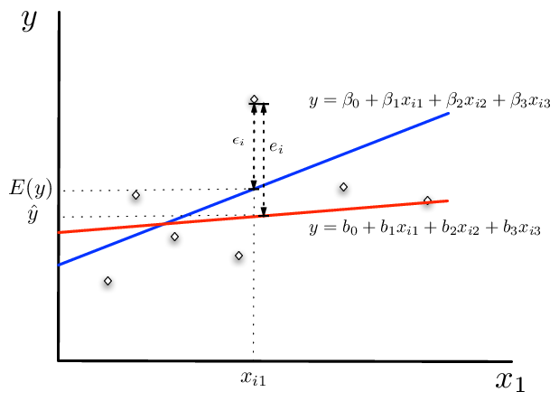
Fig. 1 Predicted (\(e_i\)) and actual (\(\epsilon_i\)) errors
The least squares estimator
The least squares is the most commonly used criteria for fitting our sample regression line to the data. Building on our matrix algebra work from earlier, we can derive the least squares estimator. The intuition behind the least squares estimator is that it seeks to minimize the sum of squared errors across the sample in the model. Recalling that the error for the sample equation is
The sum of squares criteria seeks to find an estimated value for each element of \(\mathbf{b}\) that minimizes
Denoting the set of independent variables for observation \(i\) as \(\mathbf{x_i}=\begin{bmatrix} 1 & x_{i1} & x_{i2} & x_{i3} \end{bmatrix}_{1 \times 4}\) and the vector
we can rewrite equation (4) as
Notice that defining the parameter vector as a \(4 \times 1\) column vector is necessary for conformability of the matrix multiplication operation.
We can also write the sum of squares as a matrix multiplication operation. We are now in a position to write the minimization problem in linear algebra notation. Using the foil method and noting the rules for multiplication of matrices, yields
Simplify further and recalling that \((AB)^{\prime}=B^{\prime}A^{\prime}\),
The necessary conditions for a minimum is 1:
To obtain this result, one must take note of the rule for matrix derivatives outlined in Green on page 981. Important for this problem is the property that for a matrix \(\mathbf{x}\) and \(\mathbf{y}\) and the product \(M=\mathbf{x}'\mathbf{y}\), \(\frac{\partial{M}}{\partial{\mathbf{y}}}=\mathbf{x}\). Simplifying further, the first order condition from equation (5),
Premultiplying both sides by \(\mathbf{(x'x)}^{-1}\) gives
or
which is the ordinary least squares estimator for the population parameters, \(\beta\).
Some Statistical Properties
Recall the assumptions in the classic multiple regression model:
Linearity between \(y_i\) and \(\mathbf{x_i}\)
There is no linear relationships between the columns in the matrix \(\mathbf{x}\)
Exogeneity of the independent variables: \(E[\epsilon_i|x_{j1},x_{j2},\ldots,x_{j3}]=0\), for all \(j\). This condition ensures that the independent variables for observation i, or for any other observation are not useful for predicting the disturbance terms in the model.
Homoskedasticity and no autocorrelation: \(E[\epsilon_i|\epsilon_j] \hspace{.05in}\forall j\in n\) and share the same variance \(\sigma^2\).
The independent variables may be a mixture of constants and random variables.
Disturbance terms are normally distributed, and given condition (3) and (4): \(\mathbf{\epsilon} \sim N(0,\sigma^2 I)\)
Unbiased Estimation
Recalling that the ordinary least squares estimator is
show that it is an unbiased estimator of \(\mathbf{\beta}\). Recalling from equation , We can make the following substitution for \(y\)
Taking expectations of both sides conditional on \(\mathbf{x}\),
Given assumption (3), the second term is zero, so that
Since, this holds for any values of \(\mathbf{x}\) drawn from the population,
The Variance of \(\mathbf{b}\)
The variance of our estimator \(\mathbf{b}\) is also of interest. Consider
which is equal to
substituting in for y as \(\mathbf{x \beta + \epsilon}\), the preceding equation equals
Taking note that \(\mathbf{E[\epsilon \epsilon'|x]}=\sigma^2I\) and that \(\mathbf{(x'x)^{-1}}\) is symmetric, we have
since \(\sigma^2\) is a scalar, we can pull it out of this expression to finally get our result after some simplification:
If the independent variables are non-stochastic, we have the unconditional variance of \(\mathbf{b}\) as
or, if not the variance of \(\mathbf{b}\) is
Statistical Inference
Having seen how to recover the estimated parameters and variance/covariance matrix of the parameters, it is necessary to estimate the unknown population variance of the errors \(\sigma^2\). If the true \(\mathbf{\beta}\) parameters were known, then \(\sigma^2\) could easily be computed as
in a population of \(N\) individuals. However, \(\sigma^2\) can be estimated using \(\mathbf{e=y-xb}\) in place of \(\mathbf{\epsilon}\) in the preceding equation
where \(n\) is the number of observations in the sample and \(K\) is the number of elements in the vector \(\mathbf{b}\) (referred to as degrees of freedom and is equal to the number of estimated parameters). With that, we now have the estimated variance/covariance matrix of the estimated parameters needed for statistical inference
Standard errors for each estimated parameter in \(\mathbf{b}\) can be recovered from this matrix. Suppose that we estimate a simple model and find that
the diagonal elements, highlited in yellow can be used to construct the standard errors or the coefficients. For example, the standard error of \(b_0\), assumed to be the constant term as it is the first element of \(\mathbf{b}\), would be \(\sqrt{s^2 \times 0.0665}\). Denoting the diagonal element for parameter k in \(\mathbf{(x'x)^{-1}}\) as \(S_{kk}\), we can write the standard error of \(b_k\) as
t-statistics (for the null hypothesis that \(\beta_k=0\)) can then be easily calculated as the parameter divided by the standard error:
and are distributed with n-K degrees of freedom.
Heteroskedasticity and Robust Standard Errors
From Econ 308, you probably recall the discussion about heteroskedasticity. This occurs when the variance of the model error is systematically related to the underlying data in the model. Consider Fig. 2. Notice that the slope of the line can be estimated without problem using OLS. However, assuming constant variance for the error term will lead to bad standard errors, because the deviations from the regression line (the errors) get larger as education levels increase.
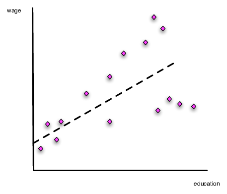
Fig. 2 Heteroskedasticity in the Ordinary Least Squares Model
Testing for Heteroskedasticity
In Econometrics you learned how to conduct the Breusch-Pagan test. The basic intuition of this test is to examine directly if any of the independent variables can systematically explain the errors in the model.
[Step 1:] Estimate the regression of interest (\(\mathbf{y=xb+\epsilon}\)) and recover \(\mathbf{e=y-xb}\), the predicted residuals, and \(\mathbf{\hat{y}=xb}\)
[Step 2:] Using the squared residuals, calculate \(\mathbf{r}=\frac{diagonal(\mathbf{ee'})}{\frac{1}{N}(\mathbf{y-xb})'(\mathbf{y-xb})}\)
[Step 3:] Estimate the regression \(\mathbf{r=\hat{y} \delta +v}\). And recover the model or explained sum of squares (stata terms this the model sum of squares): \(ESS=(\mathbf{\hat{r}}-\bar{r})'(\mathbf{\hat{r}}-\bar{r})\)
[Step 4:] Using the Explained Sum of Squares, the test statistic \(ESS/2\) is distributed \(\chi^2(1)\) for the NULL hypothesis of no heteroskedasticity.
This test has the null hypothesis of no heteroskedasticity. 2
Correcting Standard Errors in the Presence of Heteroskedasticity
If heteroskedasticity is a problem then the OLS assumption (4) is violated and while our parameter estimates are unbiased, our estimated standard errors are not correct. The intuition of this approach follows from equation (6). Rather than assuming \(E[\epsilon\epsilon']=\sigma^2 I\), we assume
where \(\mathbf{V}\) is an \(N \times N\) matrix having diagonal elements equal to \(\sigma^2_i=(y_i-\mathbf{x}_i \mathbf{b})^2\), allowing each observation’s error to effectively have their own variance.
As in the basic OLS framework, we use the estimated errors to help us estimate the non-zero elements of V. As before, calculate the model errors equal to
Computing the estimated variance covariance matrix of the residuals as
where the \(diagonal\) operator in the above expression sets off diagonal elements to zero. It is worthwhile comparing the estimated variance-covariance matrices of the errors more closely. For the OLS model, we have
whereas in the robust version of the covariance matrix we have
where \(s_i=y_i-\mathbf{x}_i \mathbf{b}\).
Given our estimate an estimate for \(E[\epsilon \epsilon']\) that better deals with the problem of heteroskedasticity, we can substitute our new estimate into equation (6) to compute the robust variance-covariance matrix for the model parameters as
These are known as robust standard errors, White standard errors, or Huber standard errors. 3 Most economists use the term “robust”. Once this is calculated t statistics can be calculated using the methods outlined above. Standard errors are the square roots of the diagonal elements.
The intuition of this approach is that the information about heteroskedasticity is embodied in our estimated error structure, and we use that error structure to calculate an estimated error variance (\(s^2_i\)) for each observation in the sample. In the preceding section, we averaged these across all individuals to calculate (\(s^2\)).
Clustered Standard Errors
A further complication may arise it we believe that some common characteristic across groups of individuals affect our error variance-covariance structure.
Examining the relationship amongst potentially clustered errors, we have (where \(\epsilon_{im}\) is the error for person \(i\) in group \(m\)):
Within Person Error Co-Variance: \(E[\epsilon_{im} \epsilon_{im}]= \sigma^2_i\)
Within-group Error Co-variance: \(E[\epsilon_{im} \epsilon_{jm}]= \rho_{ij|m}\)
Cross-group Error Co-Variance: \(E[\epsilon_{im} \epsilon_{jn}]= 0\)
Given this, we can approximate the variance covariance of our errors V using oru estimated errors \(\mathbf{e}\) as:
Having defined the variance-covariance matrix of our errors, we can then turn to equation (6), to calculate cluster-robust standard errors 4:
Implementation in Stata
In this section we show how to implement many of these ideas and
Stata. Note, this example uses data from a panel dataset (multiple
time periods per individual) and we arbitrarily restrict the analysis
to a cross section dataset by analyzing only records where time
is 4. We do this for demonstration purposes only since we motivate
this model for a pure cross section case. It is almost always a
horrible idea to throw away data like this, and later in the course we
will learn more about panel data techniques.
Running the OLS Model
Using ln_wage as our dependent variable, here is the code for
running a simple OLS model in Stata. Since we haven’t loaded the data
yet, let’s do that and run the model:
# start a connected stata17 session
from pystata import config
config.init('be')
config.set_streaming_output_mode('off')
%%stata
webuse set "https://rlhick.people.wm.edu/econ407/data/"
webuse tobias_koop
keep if time==4
regress ln_wage educ pexp pexp2 broken_home
. webuse set "https://rlhick.people.wm.edu/econ407/data/"
(prefix now "https://rlhick.people.wm.edu/econ407/data")

. webuse tobias_koop

. keep if time==4
(16,885 observations deleted)

. regress ln_wage educ pexp pexp2 broken_home

      Source |       SS           df       MS      Number of obs   =     1,034
-------------+----------------------------------   F(4, 1029)      =     51.36
       Model |  37.3778146         4  9.34445366   Prob > F        =    0.0000
    Residual |   187.21445     1,029  .181938241   R-squared       =    0.1664
-------------+----------------------------------   Adj R-squared   =    0.1632
       Total |  224.592265     1,033  .217417488   Root MSE        =    .42654

------------------------------------------------------------------------------
     ln_wage | Coefficient  Std. err.      t    P>|t|     [95% conf. interval]
-------------+----------------------------------------------------------------
        educ |   .0852725   .0092897     9.18   0.000     .0670437    .1035014
        pexp |   .2035214   .0235859     8.63   0.000     .1572395    .2498033
       pexp2 |  -.0124126   .0022825    -5.44   0.000    -.0168916   -.0079336
 broken_home |  -.0087254   .0357107    -0.24   0.807    -.0787995    .0613488
       _cons |   .4603326    .137294     3.35   0.001     .1909243    .7297408
------------------------------------------------------------------------------

.
Robust Standard Errors
Note that since the \(\mathbf{b}\)’s are unbiased estimators for \(\beta\), those continue to be the ones to report. However, our variance covariance matrix is
Defining \(\mathbf{e=y-xb}\),
In stata, the robust option is a very easy way to implement the robust
standard error correction. Note: this is not robust regression.
%%stata
regress ln_wage educ pexp pexp2 broken_home, robust
Linear regression                               Number of obs     =      1,034
                                                F(4, 1029)        =      64.82
                                                Prob > F          =     0.0000
                                                R-squared         =     0.1664
                                                Root MSE          =     .42654

------------------------------------------------------------------------------
             |               Robust
     ln_wage | Coefficient  std. err.      t    P>|t|     [95% conf. interval]
-------------+----------------------------------------------------------------
        educ |   .0852725   .0099294     8.59   0.000     .0657882    .1047568
        pexp |   .2035214   .0226835     8.97   0.000     .1590101    .2480326
       pexp2 |  -.0124126   .0022447    -5.53   0.000    -.0168173   -.0080079
 broken_home |  -.0087254   .0312381    -0.28   0.780     -.070023    .0525723
       _cons |   .4603326   .1315416     3.50   0.000     .2022121     .718453
------------------------------------------------------------------------------
The bootstrapping approach to robust standard errors
Given the advent of very fast computation even with laptop computers, we
can use boostrapping to correct our standard errrors for any non-iid
error process. In Stata, we just run (for 1000 replicates) using the following code.
I believe this is doing what is called a parametric bootstrap
(confidence intervals assume normality).
%%stata
regress ln_wage educ pexp pexp2 broken_home, vce(bootstrap,rep(1000))
(running regress on estimation sample)

Bootstrap replications (1,000)
----+--- 1 ---+--- 2 ---+--- 3 ---+--- 4 ---+--- 5
..................................................    50
..................................................   100
..................................................   150
..................................................   200
..................................................   250
..................................................   300
..................................................   350
..................................................   400
..................................................   450
..................................................   500
..................................................   550
..................................................   600
..................................................   650
..................................................   700
..................................................   750
..................................................   800
..................................................   850
..................................................   900
..................................................   950
.................................................. 1,000

Linear regression                                       Number of obs =  1,034
                                                        Replications  =  1,000
                                                        Wald chi2(4)  = 252.66
                                                        Prob > chi2   = 0.0000
                                                        R-squared     = 0.1664
                                                        Adj R-squared = 0.1632
                                                        Root MSE      = 0.4265

------------------------------------------------------------------------------
             |   Observed   Bootstrap                         Normal-based
     ln_wage | coefficient  std. err.      z    P>|z|     [95% conf. interval]
-------------+----------------------------------------------------------------
        educ |   .0852725   .0100503     8.48   0.000     .0655743    .1049707
        pexp |   .2035214    .022688     8.97   0.000     .1590538     .247989
       pexp2 |  -.0124126   .0022409    -5.54   0.000    -.0168047   -.0080205
 broken_home |  -.0087254   .0320888    -0.27   0.786    -.0716183    .0541676
       _cons |   .4603326   .1340845     3.43   0.001     .1975318    .7231333
------------------------------------------------------------------------------
We will return to why this works later in the course.
Testing for Heteroskedasticity
The two dominant heteroskedasticity tests are the White test and the Cook-Weisberg (both Breusch Pagan tests). The White test is particularly useful if you believe the error variances have a potentially non-linear relationship with model covariates. For stata, we need to make sure the basic OLS regression (rather than robust) is run just prior to these commands and then we can use:
%%stata
quietly regress ln_wage educ pexp pexp2 broken_home
imtest, white
. quietly regress ln_wage educ pexp pexp2 broken_home

. imtest, white

White's test
H0: Homoskedasticity
Ha: Unrestricted heteroskedasticity

   chi2(12) =  29.20
Prob > chi2 = 0.0037

Cameron & Trivedi's decomposition of IM-test

--------------------------------------------------
              Source |       chi2     df         p
---------------------+----------------------------
  Heteroskedasticity |      29.20     12    0.0037
            Skewness |      14.14      4    0.0068
            Kurtosis |      16.19      1    0.0001
---------------------+----------------------------
               Total |      59.53     17    0.0000
--------------------------------------------------

.
Stata’s imtest allows you to specify more esoteric forms of
heteroskedasticity. A more basic test outlined in Testing for Heteroskedasticity, that assumes
heteroskedastity is a linear function of the \(\mathbf{x}\)’s- is the
Cook-Weisberg Breusch Pagan test. In Stata, we use
%%stata
hettest
Breusch–Pagan/Cook–Weisberg test for heteroskedasticity
Assumption: Normal error terms
Variable: Fitted values of ln_wage

H0: Constant variance

    chi2(1) =  19.57
Prob > chi2 = 0.0000
- 1
As pointed out in Greene, one additional condition is necessary to ensure that we have minimized the sum of square distances for our sample. Our first order condition finds either a minimum or maximum sum of squares distances, to ensure a minimum, \(\frac{\partial{S}}{\partial{\mathbf{b}}\partial{\mathbf{b'}}}\) must be a positive definite matrix. This is the matrix analog to ensure that the function is convex with respect to changes in the parameters. Green shows that this is indeed the case so we can safely ignore checking for this condition.
- 2
A stronger version of the test, termed White’s Test is preferred to the Breusch-Pagan Cook Weissberg test shown here. See the companion document for more information.
- 3
It is important to note that Stata scales each element of \(\hat{V}\) by \(\frac{N}{N-k}\) to reduce the bias of the estimated variance covariance matrix for small sample corrections.
- 4
Stata scales \(\mathbf{\hat{V}}_{cluster}\) by \(\frac{M}{M-1}\frac{N-1}{N-K}\) for small sample corrections when calculating standard errors.