Companion for OLS Chapter
This page has been moved to https://econ.pages.code.wm.edu/407/notes/docs/index.html and is no longer being maintained here.
This companion to the OLS Chapter shows how to implement the models in both Stata and R. Unless stated otherwise, the code shown here is for R. Note, we use a panel dataset (multiple time periods per individual) and arbitrarily restrict our analysis to a cross section dataset by analyzing only records where time is 4. We do this for demonstration purposes only- it is usually a horrible idea to throw away data like this, and later in the course we will learn more about panel data techniques.
# allows us to open stata datasets
library(foreign)
# for heteroskedasticity corrected variance/covariance matrices
library(sandwich)
# for White Heteroskedasticity Test
library(lmtest)
# for bootstrapping
library(boot)
# for column percentiles
library(matrixStats)
tk.df = read.dta("https://rlhick.people.wm.edu/econ407/data/tobias_koop.dta")
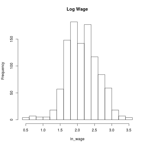
tk4.df = subset(tk.df, time == 4)
histwage <- hist(tk4.df$ln_wage,main = "Log Wage",xlab="ln_wage")
The OLS Model
Using ln_wage as our dependent variable, here is the code for running a simple OLS model in stata and R. First in Stata. Since we haven't loaded the data yet, let's do that and run the model:
webuse set "https://rlhick.people.wm.edu/econ407/data/"
webuse tobias_koop
keep if time==4
regress ln_wage educ pexp pexp2 broken_home
set more off
(prefix now "https://rlhick.people.wm.edu/econ407/data")
(16,885 observations deleted)

      Source |       SS           df       MS      Number of obs   =     1,034
-------------+----------------------------------   F(4, 1029)      =     51.36
       Model |  37.3778146         4  9.34445366   Prob > F        =    0.0000
    Residual |   187.21445     1,029  .181938241   R-squared       =    0.1664
-------------+----------------------------------   Adj R-squared   =    0.1632
       Total |  224.592265     1,033  .217417488   Root MSE        =    .42654

------------------------------------------------------------------------------
     ln_wage |      Coef.   Std. Err.      t    P>|t|     [95% Conf. Interval]
-------------+----------------------------------------------------------------
        educ |   .0852725   .0092897     9.18   0.000     .0670437    .1035014
        pexp |   .2035214   .0235859     8.63   0.000     .1572395    .2498033
       pexp2 |  -.0124126   .0022825    -5.44   0.000    -.0168916   -.0079336
 broken_home |  -.0087254   .0357107    -0.24   0.807    -.0787995    .0613488
       _cons |   .4603326    .137294     3.35   0.001     .1909243    .7297408
------------------------------------------------------------------------------
In R, we use
ols.lm = lm(ln_wage~educ + pexp + pexp2 + broken_home, data=tk4.df)
summary(ols.lm)
Call:
lm(formula = ln_wage ~ educ + pexp + pexp2 + broken_home, data = tk4.df)

Residuals:
     Min       1Q   Median       3Q      Max
-1.69490 -0.24818 -0.00079  0.25417  1.51139

Coefficients:
             Estimate Std. Error t value Pr(>|t|)
(Intercept)  0.460333   0.137294   3.353 0.000829 ***
educ         0.085273   0.009290   9.179  < 2e-16 ***
pexp         0.203521   0.023586   8.629  < 2e-16 ***
pexp2       -0.012413   0.002283  -5.438 6.73e-08 ***
broken_home -0.008725   0.035711  -0.244 0.807020
---
Signif. codes:  0 ‘***’ 0.001 ‘**’ 0.01 ‘*’ 0.05 ‘.’ 0.1 ‘ ’ 1

Residual standard error: 0.4265 on 1029 degrees of freedom
Multiple R-squared:  0.1664,	Adjusted R-squared:  0.1632
F-statistic: 51.36 on 4 and 1029 DF,  p-value: < 2.2e-16
Robust Standard Errors
Note that since the \(\mathbf{b}\)'s are unbiased estimators for \(\beta\), those continue to be the ones to report. However, our variance covariance matrix is \[ VARCOV_{HC1} = \mathbf{(x'x)^{-1}V(x'x)^{-1}} \]
Defining \(\mathbf{e=y-xb}\), \[ \mathbf{V} = diag(\mathbf{ee}') \]
In stata, the robust option is a very easy way to implement the robust standard error correction. Note: this is not robust regression.
regress ln_wage educ pexp pexp2 broken_home, robust
Linear regression                               Number of obs     =      1,034
                                                F(4, 1029)        =      64.82
                                                Prob > F          =     0.0000
                                                R-squared         =     0.1664
                                                Root MSE          =     .42654

------------------------------------------------------------------------------
             |               Robust
     ln_wage |      Coef.   Std. Err.      t    P>|t|     [95% Conf. Interval]
-------------+----------------------------------------------------------------
        educ |   .0852725   .0099294     8.59   0.000     .0657882    .1047568
        pexp |   .2035214   .0226835     8.97   0.000     .1590101    .2480326
       pexp2 |  -.0124126   .0022447    -5.53   0.000    -.0168173   -.0080079
 broken_home |  -.0087254   .0312381    -0.28   0.780     -.070023    .0525723
       _cons |   .4603326   .1315416     3.50   0.000     .2022121     .718453
------------------------------------------------------------------------------
Implementing this in R, we can use the sandwich package's `vcovHC` function with the `HC1` option (stata default):
VARCOV = vcovHC(ols.lm, 'HC1')
se = sqrt(diag(VARCOV))
print(se)
(Intercept)        educ        pexp       pexp2 broken_home
0.131541623 0.009929445 0.022683530 0.002244678 0.031238081
Note that the F-statistic reported by the R OLS result above is inappropriate in the presence of heteroskedasticity. We need to use a different form of the F test. Stata does this automatically. In R, we need to use waldtest for the correct model F statistic:
waldtest(ols.lm, vcov = vcovHC(ols.lm,'HC1'))
Wald test

Model 1: ln_wage ~ educ + pexp + pexp2 + broken_home
Model 2: ln_wage ~ 1
  Res.Df Df     F    Pr(>F)
1   1029
2   1033 -4 64.82 < 2.2e-16 ***
---
Signif. codes:  0 ‘***’ 0.001 ‘**’ 0.01 ‘*’ 0.05 ‘.’ 0.1 ‘ ’ 1
So far, we have gotten R to provide us with the correct robust standard error regression results but it isn't in a single table. To put it together for printing, use
# copy summary object
robust.summ = summary(ols.lm)
# overwrite all coefficients with robust counterparts
robust.summ$coefficients = unclass(coeftest(ols.lm, vcov. = VARCOV))
# overwrite f stat with correct robust value
f_robust = waldtest(ols.lm, vcov = VARCOV)
robust.summ$fstatistic[1] = f_robust$F[2]
print(robust.summ)
Call:
lm(formula = ln_wage ~ educ + pexp + pexp2 + broken_home, data = tk4.df)

Residuals:
     Min       1Q   Median       3Q      Max
-1.69490 -0.24818 -0.00079  0.25417  1.51139

Coefficients:
             Estimate Std. Error t value Pr(>|t|)
(Intercept)  0.460333   0.131542   3.500 0.000486 ***
educ         0.085273   0.009929   8.588  < 2e-16 ***
pexp         0.203521   0.022684   8.972  < 2e-16 ***
pexp2       -0.012413   0.002245  -5.530 4.06e-08 ***
broken_home -0.008725   0.031238  -0.279 0.780057
---
Signif. codes:  0 ‘***’ 0.001 ‘**’ 0.01 ‘*’ 0.05 ‘.’ 0.1 ‘ ’ 1

Residual standard error: 0.4265 on 1029 degrees of freedom
Multiple R-squared:  0.1664,	Adjusted R-squared:  0.1632
F-statistic: 64.82 on 4 and 1029 DF,  p-value: < 2.2e-16
The bootstrapping approach to robust standard errors
Given the advent of very fast computation even with laptop computers, we can use boostrapping to correct our standard errrors for any non-iid error process. In R, we run this (and by asking for percentiles) to get non-parametric bootstrap estimates for confidence intervals:
bs_ols <- function(formula, data, indices) {
  d <- data[indices,] # allows boot to select sample
  fit <- lm(formula, data=d) # runs the model for this sample
  return(coef(fit)) # returns coefficients
}

results <- boot(data=tk4.df, statistic=bs_ols,
        R=1000, formula=ln_wage~educ + pexp + pexp2 + broken_home)
From that we can extract the 95\% confidence intervals from the 1000 replicates.
ci_mat = colQuantiles(results$t,probs=c(.025,.975))
ci = data.frame(ci_mat,row.names=c("Intercept","educ","pexp","pexp2","broken_home"))
colnames(ci) = c("2.5%","97.5%")
print(ci)
                   2.5%        97.5%
Intercept    0.19939776  0.714556678
educ         0.06565962  0.104340132
pexp         0.16128174  0.249996019
pexp2       -0.01696095 -0.008148125
broken_home -0.07249099  0.056744122
In Stata, we just run (for 1000 replicates) using the following code. I believe this is doing what is called a parametric bootstrap (confidence intervals assume normality). As you can see, the Stata method is much easier to implement.
regress ln_wage educ pexp pexp2 broken_home, vce(bootstrap,rep(1000))
(running regress on estimation sample)

Bootstrap replications (1000)
----+--- 1 ---+--- 2 ---+--- 3 ---+--- 4 ---+--- 5
..................................................    50
..................................................   100
..................................................   150
..................................................   200
..................................................   250
..................................................   300
..................................................   350
..................................................   400
..................................................   450
..................................................   500
..................................................   550
..................................................   600
..................................................   650
..................................................   700
..................................................   750
..................................................   800
..................................................   850
..................................................   900
..................................................   950
..................................................  1000

Linear regression                               Number of obs     =      1,034
                                                Replications      =      1,000
                                                Wald chi2(4)      =     252.66
                                                Prob > chi2       =     0.0000
                                                R-squared         =     0.1664
                                                Adj R-squared     =     0.1632
                                                Root MSE          =     0.4265

------------------------------------------------------------------------------
             |   Observed   Bootstrap                         Normal-based
     ln_wage |      Coef.   Std. Err.      z    P>|z|     [95% Conf. Interval]
-------------+----------------------------------------------------------------
        educ |   .0852725   .0100503     8.48   0.000     .0655743    .1049707
        pexp |   .2035214    .022688     8.97   0.000     .1590538     .247989
       pexp2 |  -.0124126   .0022409    -5.54   0.000    -.0168047   -.0080205
 broken_home |  -.0087254   .0320888    -0.27   0.786    -.0716183    .0541676
       _cons |   .4603326   .1340845     3.43   0.001     .1975318    .7231333
------------------------------------------------------------------------------
Testing for Heteroskedasticity
The two dominant heteroskedasticity tests are the White test and the Cook-Weisberg (both Breusch Pagan tests). The White test is particularly useful if you believe the error variances have a potentially non-linear relationship with model covariates. For stata, we need to make sure the basic OLS regression (rather than robust) is run just prior to these commands and then we can use:
quietly regress ln_wage educ pexp pexp2 broken_home
imtest, white
White's test for Ho: homoskedasticity
         against Ha: unrestricted heteroskedasticity

         chi2(12)     =     29.20
         Prob > chi2  =    0.0037

Cameron & Trivedi's decomposition of IM-test

---------------------------------------------------
              Source |       chi2     df      p
---------------------+-----------------------------
  Heteroskedasticity |      29.20     12    0.0037
            Skewness |      14.14      4    0.0068
            Kurtosis |      16.19      1    0.0001
---------------------+-----------------------------
               Total |      59.53     17    0.0000
---------------------------------------------------
In R, we perform the White test by:
bptest(ols.lm,ln_wage ~ educ*pexp + educ*pexp2 + educ*broken_home + pexp*pexp2 + pexp*broken_home +
         pexp2*broken_home + I(educ^2) + I(pexp^2) + I(pexp2^2) + I(broken_home^2),data=tk4.df)
	studentized Breusch-Pagan test

data:  ols.lm
BP = 29.196, df = 12, p-value = 0.003685
Notice that in R, we need to specify the form of the heteroskedasticity. To mirror the White test, we include interaction and second order terms. Both Stata's imtest and R's bptest allow you to specify more esoteric forms of heteroskedasticity, although in R it is more apparent since we have to specify the form of the heteroskedasticity for the test to run.
A more basic test- one assuming that heteroskedastity is a linear function of the \(\mathbf{x}\)'s- is the Cook-Weisberg Breusch Pagan test.
In stata, we use
hettest
Breusch-Pagan / Cook-Weisberg test for heteroskedasticity
         Ho: Constant variance
         Variables: fitted values of ln_wage

         chi2(1)      =    19.57
         Prob > chi2  =   0.0000
R doesn't implement this test directly. But it can be performed manually following these steps:
- Recover residuals as above, denote as \(\mathbf{e}\)
- square the residuals by the sqare root of mean squared residuals:
\[ \mathbf{r} = \frac{diagonal(\mathbf{ee}')}{\sqrt{\mathbf{e'e}/N}} \]
- Run the regression \(\mathbf{r} = \gamma_0 + \gamma_1 \mathbf{xb} + \mathbf{v}\). Recall that \(\mathbf{xb} = \mathbf{\hat{y}}\).
- Recover ESS defined as
\[ ESS = (\mathbf{\hat{r}} - \bar{r})'(\hat{\mathbf{r}} - \bar{r}) \]
- ESS/2 is the test statistic distributed \(\chi^2_{(1)}\)
r = diag(tcrossprod(ols.lm$residuals))/mean(diag(tcrossprod(ols.lm$residuals)))
xb = ols.lm$fitted.values
het_ols_results = lm(r~xb)
mss = crossprod(het_ols_results$fitted.values - mean(r))
cw = mss/2
sprintf("BP / Cook-Weisberg score for heterosk.: %2.3f distributed chi2 with %d df.",cw,1)
[1] "BP / Cook-Weisberg score for heterosk.: 19.572 distributed chi2 with 1 df."