ECON 407: Companion to Maximum Likelihood
This page has been moved to https://econ.pages.code.wm.edu/407/notes/docs/index.html and is no longer being maintained here.
This companion to the maximum likelihood discussion shows how to implement many of our topics in R and Stata.
The maximum likelihood method seeks to find model parameters \(\pmb{\theta}^{MLE}\) that maximizes the joint likelihood (the likelihood function- \(L\)) of observing \(\mathbf{y}\) conditional on some structural model that is a function of independent variables \(\mathbf{x}\) and model parameters \(\pmb{\theta}^{MLE}\): \[ \pmb{\theta}^{MLE} = \underset{\pmb{\theta}}{\operatorname{max}} L = \underset{\pmb{\theta}}{\operatorname{max}} \prod_{i=1}^N prob(y_i|\mathbf{x}_i,\pmb{\theta}) \] In a simple ordinary least squares setting with a linear model, we have the model parameters \(\pmb{\theta}=[\pmb{\beta},\sigma]\) making the likelihood function \[ prob(y_i|\mathbf{x}_i,\pmb{\beta},\sigma) = \frac{1}{\sqrt{2\sigma^2 \pi}}e^{\frac{-(y_i - \mathbf{x}_i\pmb{\beta})^2}{2\sigma^2}} \] Typically, for computational purposes we work with the log-likelihood function rather than the the likelihood. This is \[ log(L) = \sum_{i=1}^N log(prob(y_i|\mathbf{x}_i,\pmb{\theta})) \]
In the code below we show how to implement a simple regression model using generic maximum likelihood estimation in stata and R. While this is a toy example with existing estimators in stata (regress) and R (lm), we develop the example here for demonstration purposes.
We'll be estimating a standard OLS model using maximum likelihood. For bench-marking purposes, the standard OLS estimation results in stata are given below:
webuse set "https://rlhick.people.wm.edu/econ407/data"
webuse tobias_koop
keep if time==4
regress ln_wage educ pexp pexp2 broken_home
set more off
(prefix now "https://rlhick.people.wm.edu/econ407/data")
(16,885 observations deleted)

      Source |       SS           df       MS      Number of obs   =     1,034
-------------+----------------------------------   F(4, 1029)      =     51.36
       Model |  37.3778146         4  9.34445366   Prob > F        =    0.0000
    Residual |   187.21445     1,029  .181938241   R-squared       =    0.1664
-------------+----------------------------------   Adj R-squared   =    0.1632
       Total |  224.592265     1,033  .217417488   Root MSE        =    .42654

------------------------------------------------------------------------------
     ln_wage |      Coef.   Std. Err.      t    P>|t|     [95% Conf. Interval]
-------------+----------------------------------------------------------------
        educ |   .0852725   .0092897     9.18   0.000     .0670437    .1035014
        pexp |   .2035214   .0235859     8.63   0.000     .1572395    .2498033
       pexp2 |  -.0124126   .0022825    -5.44   0.000    -.0168916   -.0079336
 broken_home |  -.0087254   .0357107    -0.24   0.807    -.0787995    .0613488
       _cons |   .4603326    .137294     3.35   0.001     .1909243    .7297408
------------------------------------------------------------------------------
Maximum Likelihood in Stata
To setup the model, we need to program in the normal log-likelihood function. Here is the code defining the likelihood function and estimating the maximum likelihood model:
program define ols_mle
 * This program defines the contribution of the likelihood function
 * for each observation in a simple OLS model
   args lnf xb sigma
   qui replace `lnf' =ln(1/sqrt(2*_pi*(`sigma')^2)) - (($ML_y1 - `xb')^2)/(2*(`sigma')^2)
 end
Having defined the likelihood, use the stata maximum likelihood capabilities. Note: the code is telling the Maximum likelihood program
- we want a linear function (lf) modeling the mean
- y as a linear function of the independent variables
- sigma is modeled as a constant
ml model lf ols_mle (ln_wage=educ pexp pexp2 broken_home) (sigma:)
ml max
initial:       log likelihood =     -<inf>  (could not be evaluated)
feasible:      log likelihood = -6232.9439
rescale:       log likelihood = -1697.4414
rescale eq:    log likelihood = -722.18386
Iteration 0:   log likelihood = -722.18386
Iteration 1:   log likelihood = -606.03669
Iteration 2:   log likelihood = -583.66648
Iteration 3:   log likelihood = -583.66289
Iteration 4:   log likelihood = -583.66289

                                                Number of obs     =      1,034
                                                Wald chi2(4)      =     206.44
Log likelihood = -583.66289                     Prob > chi2       =     0.0000

------------------------------------------------------------------------------
     ln_wage |      Coef.   Std. Err.      z    P>|z|     [95% Conf. Interval]
-------------+----------------------------------------------------------------
eq1          |
        educ |   .0852725   .0092672     9.20   0.000     .0671092    .1034358
        pexp |   .2035214   .0235288     8.65   0.000     .1574058     .249637
       pexp2 |  -.0124126    .002277    -5.45   0.000    -.0168755   -.0079497
 broken_home |  -.0087254   .0356243    -0.24   0.807    -.0785477     .061097
       _cons |   .4603326   .1369617     3.36   0.001     .1918926    .7287726
-------------+----------------------------------------------------------------
sigma        |
       _cons |   .4255097   .0093569    45.48   0.000     .4071704    .4438489
------------------------------------------------------------------------------
Maximum Likelihood in R
Load data and put into an R dataframe.
library(foreign)
library(maxLik)

tk.df = read.dta("https://rlhick.people.wm.edu/econ407/data/tobias_koop.dta")
tk4.df = subset(tk.df, time == 4)
tk4.df$ones=1
attach(tk4.df)
Loading our data:
y = ln_wage
X = matrix(c(educ,pexp,pexp2,broken_home,ones),nrow = length(educ))
ols.lnlike <- function(theta) {
  if (theta[1] <= 0) return(NA)
  -sum(dnorm(y, mean = X %*% theta[-1], sd = theta[1], log = TRUE))
}
Notice, we can evaluate this function at any parameter value (where the first parameter is \(\sigma\)):
ols.lnlike(c(1,1,1,1,1,1))
1305304.09136282
Manual Optimization (the hard way)
While this method is the hard way, it demonstrates the mechanics of optimization in R. In order to find the best or optimal parameters, we use R's optim function to find the estimated parameter vector. It needs as arguments
- starting values
- optimization method (for unconstrained problems `BFGS` is a good choice)
- function to be minimized
- any data that the function needs for evaluation.
Also, we can ask `optim` to return the hessian, which we'll use for calculating standard errors. The code below calls optim on our function with starting values of 1 for all parameters c(1,.1,.1,.1,.1,.1) and uses the BFGS optimization method and asks for a hessian to be returned. This runs the maximum likelihood model and assembles results in a table:
mle_res.optim = optim(c(1,.1,.1,.1,.1,.1), method="BFGS", fn=ols.lnlike, hessian=TRUE)
# parameter estimates
b = round(mle_res.optim$par,5)
# std errors
se = round(sqrt(diag(solve(mle_res.optim$hessian))),5)
labels = c('sigma','educ','pexp','pexp2','broken_home','Constant')
tabledat = data.frame(matrix(c(labels,b,se),nrow=length(b)))
names(tabledat) = c("Variable","Parameter","Standard Error")
print(tabledat)
     Variable Parameter Standard Error
1       sigma   0.42551        0.00936
2        educ   0.08527        0.00927
3        pexp   0.20352        0.02353
4       pexp2  -0.01241        0.00228
5 broken_home  -0.00873        0.03562
6    Constant   0.46033        0.13696
Using maxLik (the easy way)
Unlike optim above, the maxLik package needs the log-likelihood value not -1*log-likelihood. So let's redefine the likelihood:
ols.lnlike <- function(theta) {
  if (theta[1] <= 0) return(NA)
  sum(dnorm(y, mean = X %*% theta[-1], sd = sqrt(theta[1]), log = TRUE))
}
# starting values with names (a named vector)
start = c(1,.1,.1,.1,.1,.1)
names(start) = c("sigma2","educ","pexp","pexp2","broken_home","Constant")
mle_res <- maxLik( logLik = ols.lnlike, start = start, method="BFGS" )
print(summary(mle_res))
--------------------------------------------
Maximum Likelihood estimation
BFGS maximization, 117 iterations
Return code 0: successful convergence
Log-Likelihood: -583.6629
6  free parameters
Estimates:
             Estimate Std. error t value  Pr(> t)
sigma2       0.181058   0.007963  22.737  < 2e-16 ***
educ         0.085273   0.009262   9.207  < 2e-16 ***
pexp         0.203521   0.023524   8.652  < 2e-16 ***
pexp2       -0.012413   0.002277  -5.452 4.99e-08 ***
broken_home -0.008725   0.035626  -0.245 0.806525
Constant     0.460333   0.136859   3.364 0.000769 ***
---
Signif. codes:  0 ‘***’ 0.001 ‘**’ 0.01 ‘*’ 0.05 ‘.’ 0.1 ‘ ’ 1
--------------------------------------------
My personal opinion is that if you do a lot of this type of work (writing custom log-likelihoods), you are better off using Matlab, R, or Python than Stata. If you use R my strong preference is to use maxLik as I demonstrate above over mle or mle2, since the latter two require that you define your likelihood function as having separate arguments for each parameter to be optimized over.
Visualizing the Likelihood Function
Let's graph likelihood for the educ coefficient, holding
- all data at observed values
- other parameters constant at optimal values
I am going to call this a "marginal log-likelihood" since we are only allowing one parameter to vary (rather than all 6). Here is what it looks like:
coeff2 = mle_res.optim$par
altcoeff <- seq(.06,.11,0.001)
LL <- NULL

# calculates the LL for various values of the education parameter
# and stores them in LL:
for (m in altcoeff) {
  coeff2[2] <- m # consider a candidate parameter value for education
  LLt <- -1*ols.lnlike(coeff2)
  LL <- rbind(LL,LLt)
}


plot(altcoeff,LL, type="l", xlab="Education Coefficient", ylab="-LogL",
     main="Marginal Log-Likelihood Function for \n Education Coefficient")

abline(v=mle_res.optim$par[2], col="red")
abline(h=mle_res.optim$value, col="red")
dev.copy(png,'/tmp/marginal_mle.png')
dev.off()
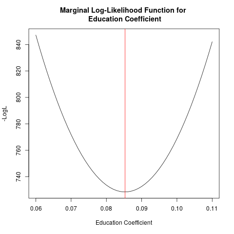
Notice that as we move away from the estimated value (the red line), the log-likelihood function declines as we lose joint probability from the estimation sample.