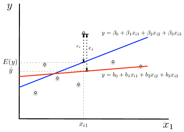
Figure 1. Disturbance Terms, Parameters, and Variable in OLS
For example, consider the population regression equation for an individual $i$
$$
\begin{equation}\label{ols:eq:popeq}
y_i=\beta_0+\beta_1 x_{i1}+\beta_2 x_{i2}+\beta_3 x_{i3} + \epsilon_i
\end{equation}
$$
where the dependent variable, $y_i$ is a function of three classes of variables:
This regression equation seeks to explain how the dependent variable, $y_i$ varies with the independent variables $x_1$, $x_2$, and $x_3$. Since we as econometric analysts can not hope to observe everything possibly affecting $y_i$, we also include disturbance terms ($\epsilon_i$) that express how individual observations deviate from the structural relationship between the dependent and independent variables.
Equation \eqref{ols:eq:popeq} can also be written using matrix notation. First, define the matrices $\mathbf{y}$ as
$$
\begin{equation}
\mathbf{y}= \begin{bmatrix}
y_1 \\
\vdots \\
y_i \\
\vdots \\
y_N \\
\end{bmatrix}_{N \times 1}
\end{equation}
$$
Notice that this vector is of dimension $N \times 1$, or N rows by 1 column.
In a similar way, we can construct the matrix of independent variable, $\mathbf{x}$ as
$$
\begin{equation}
\mathbf{x}=
\begin{bmatrix}
1 & x_{11} & x_{12} & x_{13} \\
\vdots & \vdots & \vdots & \vdots \\
1 & x_{i1} & x_{i2} & x_{i3} \\
\vdots & \vdots & \vdots & \vdots \\
1& x_{N1} & x_{N2} & x_{N3} \\
\end{bmatrix}_{N \times 4}
\end{equation}
$$
Using $\mathbf{y}$ and $\mathbf{x}$, “stack” each observation and rewrite Equation \eqref{ols:eq:popeq} as
$$
\begin{equation}
\begin{bmatrix}
y_1 \\
\vdots \\
y_i \\
\vdots \\
y_N \\
\end{bmatrix}_{N \times 1} =
\begin{bmatrix}
1 & x_{11} & x_{12} & x_{13} \\
\vdots & \vdots & \vdots & \vdots \\
1 & x_{i1} & x_{i2} & x_{i3} \\
\vdots & \vdots & \vdots & \vdots \\
1& x_{N1} & x_{N2} & x_{N3} \\
\end{bmatrix}_{N \times 4}
\times
\begin{bmatrix}
\beta_0 \\
\beta_1 \\
\beta_2 \\
\beta_3 \\
\end{bmatrix}_{4 \times 1} +
\begin{bmatrix}
\epsilon_1 \\
\vdots \\
\epsilon_i \\
\vdots \\
\epsilon_N \\
\end{bmatrix}_{N \times 1}
\end{equation}
$$
Which in compact notation can be written
$$
\begin{equation}
\mathbf{y}=\mathbf{x}\mathbf{\beta}+\mathbf{\epsilon}
\end{equation}
$$
Using matrix multiplication, we can simplify the middle term as
$$
\begin{equation}
\begin{bmatrix}
y_1 \\
\vdots \\
y_i \\
\vdots \\
y_N \\
\end{bmatrix}_{N \times 1} =
\begin{bmatrix}
\beta_0 + \beta_1 x_{11} + \beta_2 x_{12} + \beta_3 x_{13} \\
\vdots \\
\beta_0 + \beta_1 x_{i1} + \beta_2 x_{i2} + \beta_3 x_{i3} \\
\vdots \\
\beta_0 + \beta_1 x_{N1} + \beta_2 x_{N2} + \beta_3 x_{N3} \\
\end{bmatrix}_{N \times 1}
+
\begin{bmatrix}
\epsilon_1 \\
\vdots \\
\epsilon_i \\
\vdots \\
\epsilon_N \\
\end{bmatrix}_{N \times 1}
\end{equation}
$$
Further simplifying, we can use matrix addition to find
$$
\begin{equation}
\begin{bmatrix}
y_1 \\
\vdots \\
y_i \\
\vdots \\
y_N \\
\end{bmatrix}_{N \times 1} =
\begin{bmatrix}
\beta_0 + \beta_1 x_{11} + \beta_2 x_{12} + \beta_3 x_{13} + \epsilon_1 \\
\vdots \\
\beta_0 + \beta_1 x_{i1} + \beta_2 x_{i2} + \beta_3 x_{i3} + \epsilon_i \\
\vdots \\
\beta_0 + \beta_1 x_{N1} + \beta_2 x_{N2} + \beta_3 x_{N3} +\epsilon_N \\
\end{bmatrix}_{N \times 1}
\end{equation}
$$
Notice that for each observation (or row of data), we have the equivalent result as in equation \eqref{ols:eq:popeq}:
$$
\begin{equation}
y_i=\beta_0+\beta_1 x_{i1}+\beta_2 x_{i2}+\beta_3 x_{i3} +\epsilon_i
\end{equation}
$$
Since the $\beta$’s nor the disturbance terms $\epsilon_i$ in the population equation are observable, we can estimate them (call them $\mathbf{b}$). For any value of $\mathbf{b}$, we can construct the estimated values for the disturbance terms as
$$
\begin{equation}
e_i=y_i-b_0+b_1 x_{i1}+b_2 x_{i2}+b_3 x_{i3}
\end{equation}
$$
Notice that the construction of $e_i$ is purely an algebraic relationship between the $\mathbf{b}$ in the estimating equation, the independent variables, and the dependent variables. Consequently, we may want to consider a method that fits this line by choosing $\mathbf{b}$’s that in some sense minimizes the distance between the fitted line and the dependent variable.
The OLS Figure shows these various relationships between the population regression line (in blue) and the fitted regression line (in red). Notice, we have not yet said how the $\mathbf{b}$ are to be estimated yet. Both the population and the sample regression ensure that
$$
\begin{equation}\label{ols:eq:eandeps}
y_i \equiv b_0+b_1 x_{i1}+b_2 x_{i2}+b_3 x_{i3}+e_i \equiv \beta_0+\beta_1 x_{i1}+\beta_2 x_{i2}+\beta_3 x_{i3} + \epsilon_i
\end{equation}
$$
by definition. Furthermore, notice that the vector {\bf b} is an imprecise measure of the vector $\beta$. These imprecisions are reflected in the size of the disturbance term ($\epsilon_i$) versus the estimated error $e_i$ in the figure. It need not be the case that $|\epsilon_i |<| e_i |$. For example, consider a point to the left of and above the intersection between the population and the sample regression line. Therefore, for some observations in the sample, the fitted line \emph{may} have smaller error than the true regression relationship.
Figure 1. Disturbance Terms, Parameters, and Variable in OLS
The least squares is the most commonly used criteria for fitting our sample regression line to the data. Building on our matrix algebra work from earlier, we can derive the least squares estimator. The intuition behind the least squares estimator is that it seeks to minimize the sum of squared errors across the sample in the model. Recalling that the error for the sample equation is
$$
\begin{equation}
e_i=y_i-b_0-b_1 x_{i1}-b_2 x_{i2}-b_3 x_{i3}
\end{equation}
$$
The sum of squares criteria seeks to find an estimated value for each element of $\mathbf{b}$ that minimizes
$$
\begin{equation}\label{eq:sumofsq1}
\sum^{n}_{i=1}(e_i)^2=\sum^{n}_{i=1}(y_i-b_0-b_1 x_{i1}-b_2 x_{i2}-b_3 x_{i3})^2
\end{equation}
$$
Denoting the set of independent variables for observation $i$ as $\mathbf{x_i}=\begin{bmatrix} 1 & x_{i1} & x_{i2} & x_{i3} \end{bmatrix}_{1 \times 4}$
and the vector
$$
\begin{equation}
\mathbf{b}=\begin{bmatrix}
b_0 \\
b_1 \\
b_2 \\
b_3 \\
\end{bmatrix}_{4 \times 1}
\end{equation}
$$
we can rewrite equation \eqref{eq:sumofsq1} as
$$
\begin{equation}
\sum^{n}_{i=1}(e_i)^2=\sum^{n}_{i=1}(y_i-\mathbf{x_i} \mathbf{b} )^2
\end{equation}
$$
Notice that defining the parameter vector as a $4 \times 1$ column vector is necessary for conformability of the matrix multiplication operation.
We can also write the sum of squares as a matrix multiplication operation.
We are now in a position to write the minimization problem in linear algebra notation. Using the foil method and noting the rules for multiplication of matrices, yields
$$
\begin{eqnarray}
\min_b S(b)&=&\mathbf{e}’\mathbf{e}=(\mathbf{y}-\mathbf{xb})’(\mathbf{y}-\mathbf{xb}) \\
&=&\mathbf{y’y}-\mathbf{y’xb}-\mathbf{(xb)’y}+\mathbf{(xb)’xb}
\end{eqnarray}
$$
Simplify further and recalling that $(AB)^{\prime}=B^{\prime}A^{\prime}$,
$$
\begin{eqnarray}
&=&\mathbf{y’y}-\mathbf{y’xb}-\mathbf{b’x’y}+\mathbf{b’x’xb} \\
&=&\mathbf{y’y}-2\mathbf{y’xb}+\mathbf{b’x’xb}
\end{eqnarray}
$$
The necessary conditions for a minimum is1:
$$
\begin{equation}\label{ols:eq:foc}
\frac{\partial{S}}{\partial{\mathbf{b}}}=-2\mathbf{x’y}+\mathbf{2x’xb}=0
\end{equation}
$$
To obtain this result, one must take note of the rule for matrix derivatives outlined in Green on page 981. Important for this problem is the property that for a matrix $\mathbf{x}$ and $\mathbf{y}$ and the product $M=\mathbf{x}’\mathbf{y}$, $\frac{\partial{M}}{\partial{\mathbf{y}}}=\mathbf{x}$.
Simplifying further, the first order condition from equation \eqref{ols:eq:foc},
$$
\begin{equation}
\mathbf{x’y}=\mathbf{x’xb}
\end{equation}
$$
Premultiplying both sides by $\mathbf{(x’x)}^{-1}$ gives
$$
\begin{equation}
\mathbf{(x’x)}^{-1}\mathbf{x’y}=\mathbf{(x’x)}^{-1}\mathbf{x’xb}
\end{equation}
$$
or
$$
\begin{equation}
\mathbf{b}=\mathbf{(x’x)}^{-1}\mathbf{x’y}
\end{equation}
$$
which is the ordinary least squares estimator for the population parameters, $\beta$.
Recall the assumptions in the classic multiple regression model:
Recalling that the ordinary least squares estimator is
$$
\begin{equation}
\mathbf{b}=\mathbf{(x’x)}^{-1}\mathbf{x’y}
\end{equation}
$$
show that it is an unbiased estimator of $\mathbf{\beta}$. Recalling from equation \label{ols:eq:eandeps}, We can make the following substitution for y
$$
\begin{equation}
\mathbf{b}=\mathbf{(x’x)}^{-1}\mathbf{x’(x \beta + \epsilon)}
\end{equation}
$$
Taking expectations of both sides conditional on $\mathbf{x}$,
$$
\begin{equation} E[\mathbf{b}|\mathbf{x}]=\mathbf{\beta}+E[\mathbf{(x’x)}^{-1}x’\mathbf{\epsilon}]
\end{equation}
$$
Given assumption (3), the second term is zero, so that
$$
\begin{equation}
E[\mathbf{b}|\mathbf{x}]=\mathbf{\beta}
\end{equation}
$$
Since, this holds for any values of $\mathbf{x}$ drawn from the population,
$$
\begin{equation}
E[\mathbf{b}]=\mathbf{\beta}
\end{equation}
$$
The variance of our estimator $\mathbf{b}$ is also of interest. Consider
$$
\begin{equation}
Var[\mathbf{b}|\mathbf{x}]=E[(\mathbf{b}-\mathbf{\beta})(\mathbf{b}-\mathbf{\beta})’|\mathbf{x}]
\end{equation}
$$
which is equal to
$$
\begin{equation}
Var[\mathbf{b}|\mathbf{x}]=E[(\mathbf{(x’x)^{-1}x’y}-\mathbf{\beta})(\mathbf{(x’x)^{-1}x’y}-\mathbf{\beta})’|\mathbf{x}]
\end{equation}
$$
substituting in for y as $\mathbf{x \beta + \epsilon}$, the preceding equation equals
$$
\begin{eqnarray}
Var[\mathbf{b}|\mathbf{x}]&=&E[(\mathbf{(x’x)^{-1}x’(x\beta+\epsilon)}-\mathbf{\beta})(\mathbf{(x’x)^{-1}x’(x\beta+\epsilon)}-\mathbf{\beta})’|\mathbf{x}] \\
&=&E[(\mathbf{\beta + (x’x)^{-1}x’\epsilon}-\mathbf{\beta})(\mathbf{\beta+(x’x)^{-1}x’\epsilon)}-\mathbf{\beta})’|\mathbf{x}] \\
&=&E[(\mathbf{(x’x)^{-1}x’\epsilon})(\mathbf{(x’x)^{-1}x’\epsilon})’|\mathbf{x}] \\
&=&E[\mathbf{(x’x)^{-1}x’\epsilon \epsilon’x((x’x)^{-1})’}|\mathbf{x}] \\
&=&\mathbf{(x’x)^{-1}x’E[\epsilon \epsilon’|x]x((x’x)^{-1})’)} \label{ols:eq:varb}
\end{eqnarray}
$$
Taking note that $\mathbf{E[\epsilon \epsilon’|x]}=\sigma^2I$ and that $\mathbf{(x’x)^{-1}}$ is symmetric, we have
$$
\begin{equation}
Var[\mathbf{b}|\mathbf{x}]=\mathbf{(x’x)^{-1}x’\sigma^2Ix(x’x)^{-1}}
\end{equation}
$$
since $\sigma^2$ is a scalar, we can pull it out of this expression to finally get our result after some simplification:
$$
\begin{equation}
Var[\mathbf{b}|\mathbf{x}]=\mathbf{\sigma^2(x’x)^{-1}}
\end{equation}
$$
If the independent variables are non-stochastic, we have the unconditional variance of $\mathbf{b}$ as
$$
\begin{equation}
Var[\mathbf{b}]=\mathbf{\sigma^2(x’x)^{-1}}
\end{equation}
$$
or, if not the variance of $\mathbf{b}$ is
$$
\begin{equation}
Var[\mathbf{b}]=\mathbf{\sigma^2E_x[(x’x)^{-1}]}
\end{equation}
$$
Having seen how to recover the estimated parameters and variance/covariance matrix of the parameters, it is necessary to estimate the unknown population variance of the errors $\sigma^2$. If the true $\mathbf{\beta}$
parameters were known, then $\sigma^2$ could easily be computed as
$$
\begin{equation}
\sigma^2=\frac{\mathbf{\epsilon’\epsilon}}{N}=\frac{\mathbf{(y-x\beta)’(y-x\beta)}}{N}
\end{equation}
$$
in a population of $N$ individuals. However, $\sigma^2$ can be estimated using $\mathbf{e=y-xb}$ in place of $\mathbf{\epsilon}$ in the preceding equation
$$
\begin{equation}
s^2=\frac{\mathbf{e’e}}{n-K}=\frac{\mathbf{(y-xb)’(y-xb)}}{n-K}
\end{equation}
$$
where $n$ is the number of observations in the sample and $K$ is the number of elements in the vector $\mathbf{b}$ (referred to as degrees of freedom and is equal to the number of estimated parameters). With that, we now have the estimated variance/covariance matrix of the estimated parameters needed for statistical inference
$$
\begin{equation}
Var[\mathbf{b}]=\mathbf{s^2(x’x)^{-1}}
\end{equation}
$$
Standard errors for each estimated parameter in $\mathbf{b}$ can be recovered from this matrix. Suppose that we estimate a simple model and find that
$$
\require{color}
\begin{equation}
Var[\mathbf{b}]=s^2 \mathbf{(x’x)^{-1}}=
s^2 \begin{bmatrix}
\fcolorbox{blue}{yellow}{0.0665} & -0.0042 & -0.0035 & -0.0014 \\
-0.0042 & \fcolorbox{blue}{yellow}{0.5655} & 0.0591 & -0.0197 \\
-0.0035 & 0.0591 & \fcolorbox{blue}{yellow}{0.0205} & -0.0046 \\
-0.0014 & -0.0197 & -0.0046 & \fcolorbox{blue}{yellow}{0.0015}
\end{bmatrix}
\end{equation}
$$
the diagonal elements, highlited in yellow can be used to construct the standard errors or the coefficients. For example, the standard error of $b_0$, assumed to be the constant term as it is the first element of $\mathbf{b}$, would be $\sqrt{s^2 \times 0.0665}$. Denoting the diagonal element for parameter k in $\mathbf{(x’x)^{-1}}$ as $S_{kk}$, we can write the standard error of $b_k$ as
$$
\begin{equation}
s_{b_k}=\sqrt{s^2 S_{kk}}
\end{equation}
$$
t-statistics (for the null hypothesis that $\beta_k=0$) can then be easily calculated as the parameter divided by the standard error:
$$
\begin{equation}
t=\frac{b_k}{s_{b_k}}
\end{equation}
$$
and are distributed with n-K degrees of freedom.
From Econ 308, you probably recall the discussion about heteroskedasticity. This occurs when the model error is systematically related to the underlying data in the model. Consider Figure~\ref{fig:Het_Figure}. Notice that the slope of the line can be estimated without problem using OLS. However, assuming constant variance for the error term will lead to bad standard errors, because the deviations from the regression line (the errors) get larger as education levels increase.
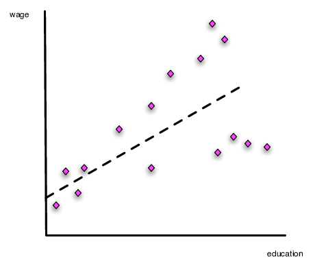
Figure 2. Heteroskedasticity in the Ordinary Least Squares Model
In Econometrics you learned how to conduct the Breusch-Pagan test. The basic intuition of this test is to examine directly if any of the independent variables can systematically explain the errors in the model.
This test has the null hypothesis of no heteroskedasticity and can be requested in stata using the command estat hettest just after the regression command.2
If heteroskedasticity is a problem then the OLS assumption (4) is violated and while our parameter estimates are unbiased, our estimated standard errors are not correct. The intuition of this approach follows from equation \eqref{ols:eq:varb}. Rather than assuming
$E[\epsilon\epsilon’]=\sigma^2 I$, we assume
$$
\begin{equation}
E[\epsilon\epsilon’]=V
\end{equation}
$$
where $\mathbf{V}$ is an $N \times N$ matrix having diagonal elements equal to $\sigma^2_i=(y_i-\mathbf{x}_i \mathbf{b})^2$, allowing each observation’s error to effectively have their own variance.
As in the basic OLS framework, we use the estimated errors to help us estimate the non-zero elements of V. As before, calculate the model errors equal to
$$
\begin{equation}
\mathbf{e}=y-x\mathbf{b}
\end{equation}
$$
Computing the estimated variance covariance matrix of the residuals as
$$
\begin{equation}
\hat{var}(\mathbf{\epsilon})=\hat{\mathbf{V}}=diagonal\left(\mathbf{ee’} \right )_{N \times N}
\end{equation}
$$
where the $diagonal$ operator in the above expression sets off diagonal elements to zero. It is worthwhile comparing the estimated variance-covariance matrices of the errors more closely. For the OLS model, we have
$$
\begin{equation}
Var(e)=s^2 \times I_{N \times N}=
\begin{bmatrix} s^2 & 0 & 0 & \ldots & 0 \\
0 & s^2 & 0 & \ldots &0 \\
0 & 0 & s^2 & \ldots & 0 \\
\vdots & \vdots & \vdots &\ddots & \vdots \\
0 & 0 & 0 & \ldots & s^2
\end{bmatrix}
\end{equation}
$$
whereas in the robust version of the covariance matrix we have
$$
\begin{equation}
Var^{robust}(e)=\hat{V}_{N \times N}=
\begin{bmatrix} s_1^2 & 0 & 0 & \ldots & 0 \\
0 & s_2^2 & 0 & \ldots &0 \\
0 & 0 & s_3^2 & \ldots & 0 \\
\vdots & \vdots & \vdots &\ddots & \vdots \\
0 & 0 & 0 & \ldots & s_N^2
\end{bmatrix}
\end{equation}
$$
where $s_i=y_i-\mathbf{x}_i \mathbf{b}$.
Given our estimate an estimate for $E[\epsilon \epsilon’]$ that better deals with the problem of heteroskedasticity, we can substitute our new estimate into equation \eqref{ols:eq:varb} to compute the robust variance-covariance matrix for the model parameters as
$$
\begin{equation}
Var^{robust}[\mathbf{b}]=\mathbf{(x’x)^{-1}x’ \hat{V} x (x’x)^{-1}}
\end{equation}
$$
These are known as robust standard errors, White standard errors, or Huber standard errors.3 Most economists use the term “robust”. Once this is calculated t statistics can be calculated using the methods outlined above. Standard errors are the square roots of the diagonal elements.
The intuition of this approach is that the information about heteroskedasticity is embodied in our estimated error structure, and we use that error structure to calculate an estimated error variance ($s^2_i$) for \emph{each} observation in the sample. In the preceding section, we averaged these across all individuals to calculate ($s^2$).
These models are very easy to implement in stata via the reg command with the robust option as demonstrated in class. To test for heteroskedasticty, use estat hettest just after your reg command.
As pointed out in Greene, one additional condition is necessary to ensure that we have minimized the sum of square distances for our sample. Our first order condition finds either a minimum or maximum sum of squares distances, to ensure a minimum, $\frac{\partial{S}}{\partial{\mathbf{b}}\partial{\mathbf{b’}}}$ must be a positive definite matrix. This is the matrix analog to ensure that the function is convex with respect to changes in the parameters. Green shows that this is indeed the case so we can safely ignore checking for this condition. ↩
Actually this command will do a non-parametric version of this test (not assuming normality of errors) and does not perfectly follow the steps outlined above, but the intuition is the same as the case presented above. ↩
It is important to note that Stata scales each element of $\hat{V}$ by $\frac{N}{N-k}$ to reduce the bias of the estimated variance covariance matrix for small sample corrections. ↩