Estimation by Maximum Likelihood
Up to now in the course, our dependent variable has been continous and distributed as $N(\mathbf{x}\beta,\sigma^2 I)$. There are many classes of problems for which the dependent variable is not normally distributed. Consider these examples:
- Whether a student is admitted ($y_i=1$) or not ($y_i=0$) to William and Mary.
- Foreign aid allocation. The US gives money to only a subset of recipient countries and therefore there are many foreign aid flows of zero. Plotting a histogram of aid flows shows many points are “stacked” on zero.
- Labor Supply: In problem set #1, over 1/3 of the sample worked zero hours.
- Duration of time on Unemployment Insurance: left skewed and not normally distributed and measured in integer counts (ie. weeks)
The important point about each of these empirical settings is that we can’t rely on OLS because our dependent variable, and hence, our model errors are not normally distributed.
A quick plot of working hours and predicted working hours- following an OLS estimation- highlite that visually speaking in Figure 1, a large spike in the histogram is occurring at zero hours. If we ignore the spike, and estimate OLS and plot predicted working hours, one sees that the model is forcing normality on our predicted dependent variable to the extent that it causes us to predict negative working hours for a sizable chunk of the sample. One might say “so what?”, as long as the estimated beta’s are ok we can use the model results for policy guidance even if model predictions are poor. To that end, consider the following monte carlo simulation.
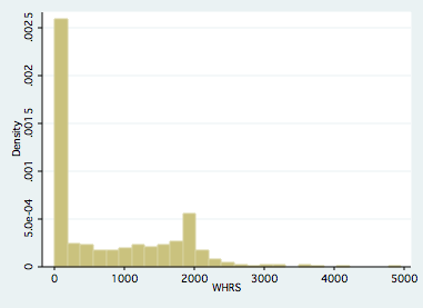
Figure 1. Observed working hours

Figure 2. Predicted working hours
Monte Carlo Simulation
I have performed a monte carlo study (code can be found here1), to investigate how close $\mathbf{b}$ is to $\beta$. With that in mind, I develop an experiment where I know the “truth” and can fully observe the population regression function for a sample of observations: $y_{N \times 1}=5+.5 x_{N \times 1} + \epsilon_{N \times 1}$. The steps of the Data Generation Process are as follows:
- Generate vector $\mathbf{x}$ of independent variables
- Generate the vector $\epsilon$ where $\epsilon$ is distributed $N(0,\sigma^2 I)$.
- Calculate ``True’‘ Dependent Variable as $y_{N \times 1}=5+.5 x_{N \times 1} + \epsilon_{N \times 1}$
- Calculate Observed Independent Variable ($Y^*$) as
- $Y^*=Y$ if $Y>7.25$
- $Y^*=7.25$ if $Y\le7.25$
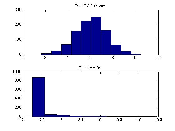
Figure 3. Dependent Variable: Monte Carlo Simulation
Using the $\mathbf{x}$ and $\mathbf{y}$, the model was estimated and the predicted errors were recovered. Recall, we must use $\mathbf{y^*}$ for constructing the predicted errors. These are depicted in the Figure below. This experiment was repeated 1000 times and the distribution of $b_1$ are shown below. Notice that the predicted error no longer looks normally distributed and is no longer symmetric. More troubling, we are systematically underestimating $\beta_1$ and there were no experiments where the estimate for $\beta_1$ was even remotely close to .5, the true value.

Figure 4. Model Error: Monte Carlo Simulation
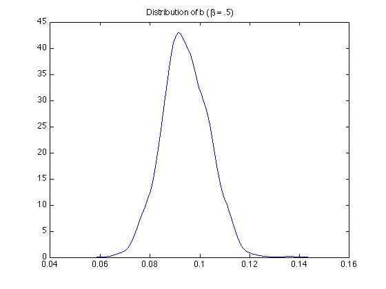
Figure 5. Estimated $b$: Monte Carlo Simulation
My example is one where very many observations were impacted by the minimum wage policy. Therefore the degree of the limited dependent variable problem plays a very important role in demonstrating the bias of the OLS parameter estimates. What we can take away from this example is that in cases like this, OLS models will perform very poorly. Since we can no longer rely on normality of the model error for constructing the structure of the model, we must turn to other techniques. One widely used technique for cases like this is called Maximum Likelihood. In this chapter we introduce the concept and give some examples.
MLE Models we will study this semester
Censoring, Truncation, and Sample Selection
The preceding example comes from problems arising from censoring or truncation. In effect part of our dependent variable is continous, but a large portion of our sample is stacked on a particular value (e.g. zero in our example)
- We don’t observe the dependent variable if the individual falls below (or above) a threshold level (truncation)
- We only observe profits if they are positive. Otherwise, they were negative or zero.
- We only observe a lower (or upper) threshold value for the dependent variable if the “true” dependent variable is below a critical value (censoring)
- The highest grade level I can assign is an “A”. Different students may have different capabilities, but all of these top students receive an “A”.}
For these kinds of problems, use the Tobit or Heckman models.
Dichotomous Choice
Consider a model of the unemployed. Some look for work and some may not. In this case the dependent variable is binary (1=Looking for work, 0=not looking for work).
In this case, we model the probability that an individual $i$ is looking for work as
$$
\begin{equation}
Prob(i \in looking) = \int^{\infty}_{-\infty}f(\mathbf{x}_i \beta|\epsilon_i)d\epsilon_i \nonumber
\end{equation}
$$
Usual assumptions about the error lead to the Probit (based on the Normal Distribution) or the Logit (based on Generalized Extreme Value Type I).
Multinomial Choice
Consider a firm siting decision among K communities. Each community may offer different tax packages, have different amenities, etc. The firm’s choice is from among one of the K sites.
Now the probability that firm i chooses community k is
$$
\begin{equation}
Prob(k|i) = \int^{\infty}_{-\infty}\ldots\int^{\infty}_{-\infty}\ldots\int^{\infty}_{-\infty}f(\mathbf{x}_{i1} \beta,\ldots,\mathbf{x}_{ik} \beta,\ldots,\mathbf{x}_{iK} \beta|\epsilon)d\epsilon \nonumber
\end{equation}
$$
Usual assumptions about the error lead to the multinomial probit (based on the Normal Distribution) or the multinomial logit (based on Generalized Extreme Value Type I).
The Maximum Likelihood Approach
Outline and Basic Steps
The idea:
- Assume a functional form and distribution for the model errors
- For each observation, construct the probability of observing the dependent variable $y_i$ conditional on model parameters $\mathbf{b}$
- Construct the Log-Likelihood Value
- Search over values for model parameters $\mathbf{b}$ that maximizes the sum of the Log-Likelihood Values
Maximum Likelihood: Formal Setup
Consider a sample $\mathbf{y}=\begin{bmatrix} y_1&\ldots&y_i&\ldots&y_N \end{bmatrix}$ from the population. The probability density function (or pdf) of the random variables $y_i$ conditioned on parameters $\theta$ is given by $f(y_i,\theta)$. The joint density of $n$ individually and identically distributed observation is $\begin{bmatrix}y_1&\ldots&y_i&\ldots&y_N\end{bmatrix}$
$$
\begin{equation}
f(\mathbf{y,\theta})=\prod^N_{i=1}f(y_i,\theta)=L(\theta|\mathbf{y})
\end{equation}
$$
is often termed the Likelihood Function and the approach is termed Maximum Likelihood Estimation (MLE).
In our excel spreadsheet example,
\begin{equation}
f(y_i,\theta) = f(y_i,\mu|\sigma^2=1) = \frac{1}{\sqrt{2 \pi \sigma^2}}e^{\frac{-(y_i-\mu)^2}{2\sigma^2}}
\end{equation}
It is common practice to work with the Log-Likelihood Function (better numerical properties for computing):
\begin{equation}
ln(L(\theta|\mathbf{y}))=\sum^N_{i=1}ln \left (\frac{1}{\sqrt{2 \pi \sigma^2}}e^{\frac{-(y_i-\mu)^2}{2\sigma^2}} \right )
\end{equation}
We showed how changing the values of $\mu$, allowed us to find the maximum log-likelihood value for the mean of our random variables $\mathbf{y}$. Hence the term maximum likelihood.
OLS and Maximum Likelihood Estimation
Recalling that in an OLS context, $\mathbf{y=xb+\epsilon}$. Put another way, $\mathbf{y}\sim N(\mathbf{x\beta,\sigma^2I})$. We can express this in a log likelihood context as
$$
\begin{equation}
f(y_i|\beta,\sigma^2,x_i) = \frac{1}{\sqrt{2 \pi \sigma^2}}e^{\frac{-(y_i-\mathbf{x_i\beta})^2}{2\sigma^2}}
\end{equation}
$$
Here we estimate the $K$ $\beta$ parameters and $\sigma^2$. By finding the $K+1$ parameter values that maximize the log likelihood function.
The maximumum likelihood estimator $b_{MLE}$ and $s_{MLE}^2$ are exactly equivalent to their OLS counterparts $b_{OLS}$ and $s_{OLS}^2$
In order to be assured of an optimal parameter vector $b_{mle}$, we need the following conditions to hold:
- $\frac{d ln (L (\theta|y,x))} {d \theta} = 0$
- $\frac{d^2 ln (L (\theta|y,x))} {d \theta^2} < 0$
When taking this approach to the data, the optimization algorithm in stata evaluates the first and second derivates of the log-likelihood function to “climb” the hill to the topmost point representing the maximum likelihood. These conditions ignore local versus global concavity issues.
Properties of the Maximum Likelihood Estimator
The Maximum Likelihood Estimator has the following properties
- Consistency: $plim(\hat{\theta})=\theta$
- Asymptotic Normality: $\hat{\theta} \sim N(\theta,I(\theta)^{-1})$
- Asymptotic Efficiency: $\hat{\theta}$ is asymptotically efficient and achieves the Rao-Cramer Lower Bound for consistent estimators (minimum variance estimator).
- Invariance: The MLE of $\delta=c(\theta)$ is $c(\hat{\theta})$ if $c(\theta)$ is a continuous differentiable function.
These properties are roughly analogous to the BLUE properties of OLS. The importance of asymptotic looms large.
Hypothesis Testing in MLE: The Information Matrix
The variance/covariance matrix of the parameters $\theta$ in an MLE framework are
$$
\begin{equation}
I(\theta) = -1 \times \frac{\partial^2 ln L(\theta)}{\partial \theta \partial \theta’}
\end{equation}
$$
and can be estimated by using our estimated parameter vector $\theta$:
$$
\begin{equation}
I(\hat{\theta}) = -1 \times \frac{\partial^2 ln L(\hat{\theta})}{\partial \hat{\theta} \partial \hat{\theta}’}
\end{equation}
$$
This matrix is our estimated variance covariance matrix for the parameters with standard errors for parameter $i$ equal to
$s.e.(i)=\sqrt{I(\hat{\theta}_{ii})^{-1}}$
Example: OLS and MLE equivalence of $Var(b)$
Suppose we estimate an OLS model over $N$ observations and $4$ parameters. The variance covariance matrix of the parameters can be written
\begin{equation}
s^2 \mathbf{(x’x)^{-1}}=
s^2 \begin{bmatrix}
0.0665 & -0.0042 & -0.0035 & -0.0014 \\
-0.0042 & 0.5655 & 0.0591 & -0.0197 \\
-0.0035 & 0.0591 & 0.0205 & -0.0046 \\
-0.0014 & -0.0197 & -0.0046 & 0.0015
\end{bmatrix}
\end{equation}
it can be shown that the first $K \times K$ rows and columns of $I(\hat{\theta})$ has the property:
\begin{equation}
I(\hat{\theta})^{-1}_{K \times K} = s^2 \mathbf{(x’x)^{-1}}
\end{equation}
Note: the last column of $I$ contains information about the variance of the parameter $s^2$. See Green 16.9.1.
Nested Hypothesis Testing
A nested hypothesis test is a test based on restrictions on some or all of our parameter estimates. Placing restrictions on our parameters, will reduce the model $R^2$ and decrease the residual sum of squares. In an OLS framework, we can use F tests based off of the Model, Total, and Error sum of squares. We don’t have that in the MLE framework because we don’t estimate model errors.
For developing similar ideas in an MLE setting, consider a restriction of the form $c(\theta)=0$. A common restriction we consider is
\begin{equation}
H_0: c(\theta)=\theta_1=\theta_2=\ldots=\theta_k=0
\end{equation}
Instead, we use one of three tests available in an MLE setting:
- Likelihood Ratio Test- Examine changes in the joint likelihood when restrictions are imposed.
- Wald Test- Look at differences across $\hat{\theta}$ and $\theta_r$ and see if they can be attributed to sampling error.
- Lagrange Multiplier Test- examine first derivative when restrictions imposed.
These are all asymptotically equivalent and all are NESTED tests.
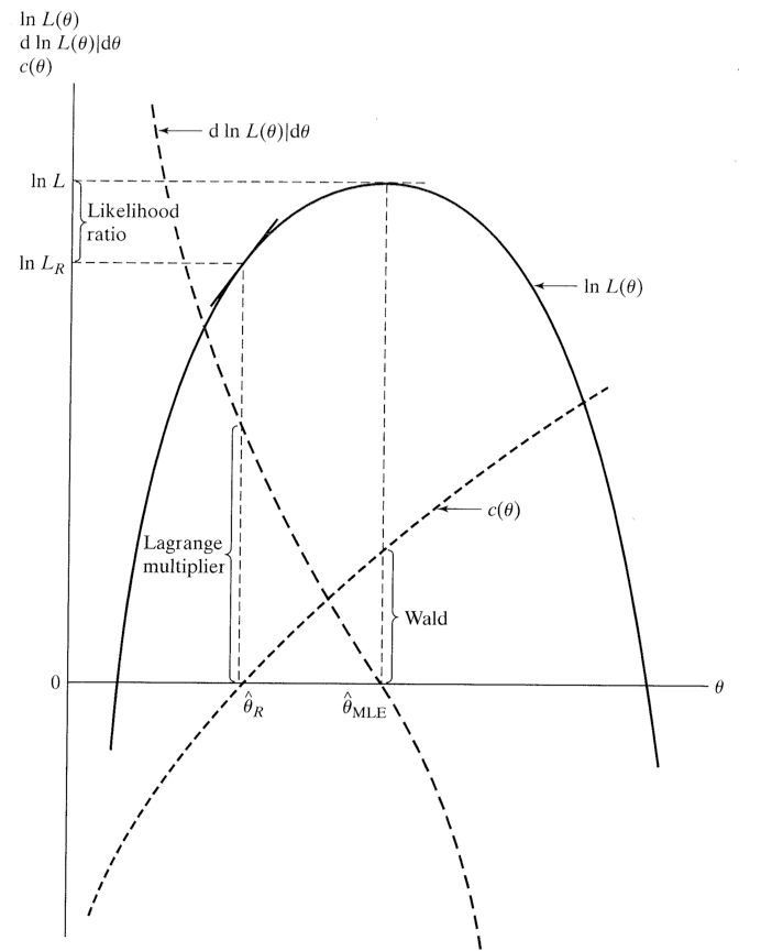
Figure 6. The likelihood function and hypothesis testing (Green).
The Likelihood Ratio Test (LR Test)
Denote $\hat{\theta}_u$ as the unconstrained value of $\theta$ estimated via MLE and let $\hat{\theta}_r$ be the constrained maximum likelihood estimator. If $\hat{L}_u$ and $\hat{L}_r$ are the likelihood function values from these parameter vectors (not Log Likelihood Values), the likelihood ratio is then
\begin{equation}\label{eq:bad}
\lambda=\frac{\hat{L}_r}{\hat{L}_u}
\end{equation}
The test statistic, $LR=-2 \times ln(\lambda)$, is distributed as $\chi^2(r)$ degrees of freedom where r are the number of restrictions. In terms of log-likelihood values, the likelihood ratio test statistic is also
\begin{equation}\label{eq:good}
LR=-2*(ln(\hat{L}_r) - ln(\hat{L}_u))
\end{equation}
This is the test we will use most often in class this semester. It is important to note that Equation $\eqref{eq:good}$ is the test statistic we use not the ratio listed above in Equation $\eqref{eq:bad}$.
The Wald Test
This test is conceptually like the Hausman test we considered in the IV sections of the course. Consider a set of linear restrictions (e.g. $R\theta=0$).
The Wald test statistic is
\begin{equation}
W=\left[ R\hat{\theta} -0 \right]’\left[R [Var.(\hat{\theta})] R’ \right ]^{-1} \left[ R\hat{\theta} -0 \right]
\end{equation}
$W$ is distributed as $\chi^2(r)$ degrees of freedom where r are the number of restrictions.
For the case of one parameter (and the restriction that it equals zero), this simplifies to
\begin{equation}
W=\frac{(\hat{\theta}-0)^2}{var(\hat{\theta})}
\end{equation}
The Lagrange Multiplier Test (LM Test)
This one considers how close the derivative of the likelihood function is to zero once restrictions are imposed. If imposing the restrictions doesn’t come at a big cost in terms of the slope of the likelihood function, then the restrictions are more likely to be consistent with the data.
The test statistic is
\begin{equation}
LM= \left ( \frac{\partial L(R\hat{\theta})}{\partial \hat{\theta}} \right )’I(\hat{\theta})^{-1} \left ( \frac{\partial L(R\hat{\theta})}{\partial \hat{\theta}} \right )
\end{equation}
$LM$ is distributed as $\chi^2(r)$ degrees of freedom where r are the number of restrictions.
For the case of one parameter (and the restriction that it equals zero), this simplifies to
\begin{equation}
LM=\frac{\left(\frac{\partial L(\hat{\theta}=0)}{\partial \hat{\theta}}\right)^2}{var(\hat{\theta})}
\end{equation}
Non-Nested Hypothesis Testing
\frametitle{Non-Nested Hypothesis Testing}
If one wishes to test hypothesis that are not nested, different procedures are needed. A common situation is comparing models (e.g. probit versus the logit). These use Information Criteria Approaches.
- Akaike Information Criterion (AIC): $-2ln(L) + 2 K$
- Bayes/Schwarz Information Criterion (BIC)]: $-2ln(L) + K ln(N)$
where $K$ is the number of parameters in the model and $N$ is the number of observations. Choosing the model based on the lowest AIC/BIC is akin to choosing the model with best adjusted $R^2$- although it isn’t necessarily based on goodness of fit, it depends on the model.
Goodness of Fit
Recall that model $R^2$ uses the predicted model error. Here, while we have errors, we don’t model them directly. Instead, there has been some work related to goodness of fit in maximum likelihood settings. McFadden’s Pseudo $R^2$ is calculated as
\begin{equation}
Psuedo \hspace{.05in} R^2=1-\frac{ln(L(\hat{\theta}))}{ln(L(\hat{\theta}_{constant}))}
\end{equation}
Some authors (Woolridge) argue that these are poor goodness of fit measures and one should tailor goodness of fit criteria for the situation one is facing.
-
Matlab Code for Monte Carlo Experiment. This code is provided for the interested student, and I don’t expect you to understand how it works, nor will you be held responsible for knowing this for any exams or problem sets.
   clc;
   clear;
   % This file shows how horribly wrong things can go when you run OLS and
   % the censoring point is highly relevant.

   sims=1000;
   obs=1000;

   b_ols=zeros(sims,2);

   for i=1:sims

   x1=2*ones(obs,1)+2*randn(obs,1);

   x=horzcat(ones(obs,1),x1);

   % Generate some random normal variates
   rand1=randn(obs,1);

   % Parameters
   b_0=5;
   b_x1=.5;

   b=vertcat(b_0,b_x1);

   % generate latent dy

   dy=x*b+rand1;

   % Observed y is truncated at 7.25
   y=dy;
   y(dy<7.25,1)=7.25;

   % RUN OLS for this monte carlo simulation and store results

   b_ols(i,:)=(inv(x’*x)*x’*y)’;

   end

   % calculate estimated errors for the last monte carlo
   % iteration for plotting.

   ehat=y-x*b_ols(end,:)’;

   subplot(2,1,1);
   [f,xi] = ksdensity(rand1);
   plot(xi,f);
   title(‘True Model Error Std. Normal’)

   subplot(2,1,2);
   [f,xi] = ksdensity(ehat);
   plot(xi,f);
   title(‘Predicted Model Error’)

   pause

   subplot(2,1,1);
   hist(dy)
   title(‘True DV Outcome’)

   subplot(2,1,2);
   hist(y)
   title(‘Observed DV’)

   pause

   subplot (1,1,1)
   % This is the density data
   [f,xi] = ksdensity(b_ols(:,2));
   plot(xi,f);
   title(‘Distribution of b (\beta = .5)’ )