ECON 407: Random Effects for Panel Data
This page has been moved to https://econ.pages.code.wm.edu/407/notes/docs/index.html and is no longer being maintained here.
In the previous chapter, we saw two approaches to dealing with recovering marginal effects in panel data. First, we showed how simple differencing in a two period example can effectively rid the model of the unobserved individual effects, albeit with some strong assumptions. We also examined the assumptions necessary to completely ignore these effects and estimate a pooled OLS regression model. These approaches are commonly used, but more can be done [1]. The literature has implemented these type of models in a number of ways, but the most prevalent are termed (1) random effects and (2) fixed effects. These terms refer to assumptions about the individual-specific constant terms \(c_i\).
The labels fixed and random effects are misleading. What matters here is the nature of the unobserved, time invariant, and individual-specific quantities. If there is a dependence between these unobserved factors and the observed independent variables we employ the fixed effects approach. If on the other hand, these effects are independent of the observed independent variables, then we use the random effects estimator. In this chapter, we focus on the random effects model. Keeping the same notation as before, let our estimating equation be
\[y_{it}=\mathbf{x}_{it}\beta+c_i+\epsilon_{it}\]
Since the impact of these unobservable factors (\(c_i\)) are put in the error structure for each individual, we assume
Assumption 1: Restrictions on the error structure
\begin{equation} \Sigma=E[v_i v'_i]=\sigma^2_\epsilon I + \sigma^2_c \psi \psi' = \begin{bmatrix} \sigma^2_\epsilon+\sigma^2_c & \sigma^2_c & \ldots & \sigma^2_c \\ \sigma^2_c & \sigma^2_\epsilon+\sigma^2_c & \ldots & \sigma^2_c \\ \vdots & & \ddots & \vdots \\ \sigma^2_c &\ldots & &\sigma^2_\epsilon+\sigma^2_c \\ \end{bmatrix} \nonumber \end{equation}where the elements of \(v\), \(v_{it}\), are defined as \(c_i+\epsilon_{it}\). Note that \(\Sigma\) is the same for all individuals in the sample. The dimensions of I and \(\psi\) (a vector whose elements are all equal to 1) are \(T \times T\) and \(T \times 1\), respectively. This defines the piece of the variance covariance matrix relevant for each individual i.
Assumption 2: The rank condition
\[rank\left ( E(x '\Omega x)\right ) = K\]
To consider what this chapter is trying to accomplish, the following figure shows the classic case that is consistent with the assumptions outlined above. Note that the "true" model shows how each set of observations (each color are four observations collected over each individual) deviates from the population regression line (in black) by the amount \(c_i\). Then, each of those points deviate around the colored lines by a random time variant unobservable component (\(\epsilon_{it} \sim N(0,\sigma^2_{\epsilon} I)\)).
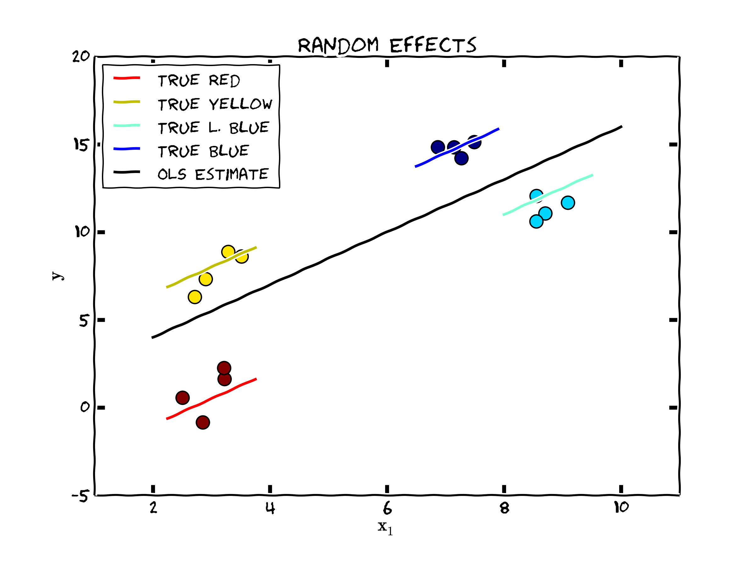
Figure 1. Data Consistent with the Random Effects Model
Estimating Parameters
To use the information embodied in this error structure for estimating \(b_{RE}\) and \(Var(b_{RE})\), we can use a weighted least squares approach, where we first estimate \(\Omega\), denoted as \(\hat{\Omega}\) and then we estimate \(b_{RE}\) as
\begin{equation} \mathbf{b_{RE}}=\mathbf{(x' \hat{\Omega}^{-1} x)}^{-1}\mathbf{x' \hat{\Omega}^{-1} y} \label{eq:re_estimator} \end{equation}Clearly to calculate Equation \(\eqref{eq:re_estimator}\) we need \(\hat{\Omega}\). By assumption,
\begin{equation} \hat{\Sigma}= \begin{bmatrix} \hat{\sigma}^2_\epsilon+\hat{\sigma}^2_c & \hat{\sigma}^2_c & \ldots & \hat{\sigma}^2_c \\ \hat{\sigma}^2_c & \hat{\sigma}^2_\epsilon+\hat{\sigma}^2_c & \ldots & \hat{\sigma^2_c} \\ \vdots & & \ddots & \vdots \\ \hat{\sigma}^2_c &\ldots & & \hat{\sigma}^2_\epsilon+\hat{\sigma}^2_c \\ \end{bmatrix}_{T \times T} \end{equation}a \(T \times T\) dimensional matrix for each individual i. \(\sigma\) follows from our assumptions above, since (noting that assuming mean zero errors for \(v_{it}\)), that
\begin{aligned} Var(v_{it})=&E[(v_i-0)^2]=E(v^2_i) \\ =&E[(\epsilon_{it}+c_i)^2] \\ =&E[\epsilon^2_{it}+2\epsilon_{it}c_i+c_i^2]\\ =&E[\epsilon^2_{it}+c_i^2] \\ =&\sigma_{\epsilon}^2+\sigma_{c}^2 \end{aligned}Noting that \(E[2\epsilon_{it}c_i]=0\) from Assumption 1. The covariance with \(v_{it+1}\)
\begin{aligned} Cov(v_{it},v_{it+1})=&E[(v_{it}-0)(v_{it+1}-0)] \\ =&E[(v_{it}v_{it+1})] \\ =&E[(\epsilon_{it}+c_i)(\epsilon_{it+1}+c_i)]\\ =&E[\epsilon_{it}\epsilon_{it+1}+\epsilon_{it}c_i+\epsilon_{it+1}c_i+c^2_i]\\ =&\sigma_c^2 \end{aligned}where the first term is zero (we assume no autocorrelation in \(\epsilon\)), and the middle two terms are zero due to Assumption 1. This leaves us with the individual specific variance assumed to be constant across all groups. These derivations explicitly show what we are imposing in this model.
It is important to note that \(E[v_{it}v_{jt}]\) and \(E[v_{it+1}v_{jt}]\) are also assumed to be zero which is implicit in the full sample variance covariance matrix for the error structure defined by
\begin{equation} \Omega=\begin{bmatrix}\label{eq:full_varcov_matrix} \Sigma & \mathbf{0}&\mathbf{0}&\ldots&\mathbf{0} \\ \mathbf{0}&\Sigma & \mathbf{0}&\ldots&\mathbf{0} \\ & & & \vdots & \\ \mathbf{0}& \mathbf{0}&\ldots&\mathbf{0} &\Sigma \end{bmatrix}_{NT \times NT} \end{equation}Since \(\Omega\) is a block diagonal matrix (having off diagonal elements not zero only when individual i and j are the same person), all information about \(\sigma^2_{c}\), which is assumed to be constant across all individuals comes from within cross section units.
To estimate these, first estimate the model using pooled OLS as in the previous chapter to recover \(\mathbf{b}_{ols}\), then find the estimated model errors as
\begin{equation} \label{eq:pooled_resids} \hat{\mathbf{v}}=\mathbf{y}-\mathbf{x} b_{ols} \end{equation}Using these we can find the overall variance of the model: \(\hat{\sigma}^2_v=\hat{\sigma}^2_\epsilon+\hat{\sigma}^2_c\) for the diagonal elements of the matrix. This is done by using the formula:
\begin{equation} \hat{\sigma}^2_v=\frac{1}{N \times T -K} \hat{\mathbf{v}}'\hat{\mathbf{v}} \nonumber \end{equation}We can also use the information contained in \(\hat{\mathbf{v}}\) to estimate the covariance in the error imparted by the individual specific unobservable factor
\begin{equation} \label{eq:var_c} \hat{\sigma}^2_c=\frac{1}{[N \times T (T-1)/2 -K]} \sum^N_{i=1} \sum^{T-1}_{t=1} \sum^{T}_{s=t+1} \hat{v}_{it}\hat{v}_{st} \end{equation}The intuition behind equation \(\eqref{eq:var_c}\) is that the complicated summation pattern takes the off diagonal elements contained in \(v\) and averages these to estimate the variance of \(c_i\). For off diagonal elements where \(i \ne j\), these elements are ignored and the equation omits these. Consider this simple example of \(N=2\) and \(T=3\) for how the estimated errors in the model (\(\hat{v}\)) are actually used for calculating \(\sigma^2_c\):
\begin{equation} \label{eq:re_example} \begin{matrix} Individual & t & s & Row,Column \\ \hline 1 & 1 & 2 & 1,2 \\ 1 & 1 & 3 & 1,3 \\ 1 & 2 & 3 & 2,3 \\ 2 & 1 & 2 & 1,2 \\ 2 & 1 & 3 & 1,3 \\ 2 & 2 & 3 & 2,3 \end{matrix} \end{equation} \begin{equation} \hat{\mathbf{v}}\hat{\mathbf{v}}'= \begin{bmatrix} \hat{v}_{11}\hat{v}_{11} & \color{blue}{\hat{v}_{11}\hat{v}_{12}} & \color{blue}{\hat{v}_{11}\hat{v}_{13}} & \hat{v}_{11}\hat{v}_{21} & \hat{v}_{11}\hat{v}_{22} & \hat{v}_{11}\hat{v}_{23} \\ \hat{v}_{12}\hat{v}_{11} & \hat{v}_{12}\hat{v}_{12} & \color{blue}{\hat{v}_{12}\hat{v}_{13}} & \hat{v}_{12}\hat{v}_{21} & \hat{v}_{12}\hat{v}_{22} & \hat{v}_{12}\hat{v}_{23} \\ \hat{v}_{13}\hat{v}_{11} & \hat{v}_{13}\hat{v}_{12} & \hat{v}_{13}\hat{v}_{13} & \hat{v}_{13}\hat{v}_{21} & \hat{v}_{13}\hat{v}_{22} & \hat{v}_{13}\hat{v}_{23} \\ \hat{v}_{21}\hat{v}_{11} & \hat{v}_{21}\hat{v}_{12} & \hat{v}_{21}\hat{v}_{13} & \hat{v}_{21}\hat{v}_{21} & \color{red}{\hat{v}_{21}\hat{v}_{22}} & \color{red}{\hat{v}_{21}\hat{v}_{23}} \\ \hat{v}_{22}\hat{v}_{11} & \hat{v}_{22}\hat{v}_{12} & \hat{v}_{22}\hat{v}_{13} & \hat{v}_{22}\hat{v}_{21} & \hat{v}_{22}\hat{v}_{22} & \color{red}{\hat{v}_{22}\hat{v}_{23}} \\ \hat{v}_{23}\hat{v}_{11} & \hat{v}_{23}\hat{v}_{12} & \hat{v}_{23}\hat{v}_{13} & \hat{v}_{23}\hat{v}_{21} & \hat{v}_{23}\hat{v}_{22} & \hat{v}_{23}\hat{v}_{23} \end{bmatrix} \nonumber \end{equation}The blue elements are included for individual 1, while the red elements are included for individual 2. Only the upper diagonal elements are used in the average because of symmetry. Also note that in our example, the denominator in \(\eqref{eq:var_c}\) is equal to \(6-K\), or the number of elements included in the summation minus the number of parameters estimated from the independent variables in the model. All other upper diagonal elements are ignored in this formula due to the constraints imposed by using equation \(\eqref{eq:full_varcov_matrix}\), even if they are not zero!! [2]
From there, it is easy to calculate \(\hat{\sigma}^2_\epsilon=\hat{\sigma}^2_v-\hat{\sigma}^2_c\), and calculate \(\hat{\Omega}\) for use in equation \(\eqref{eq:re_estimator}\).
Weighted Least Squares and the Role of \(\hat{\Omega}\)
To investigate how \(\sigma^2_c\) influences our estimates of \(\mathbf{b}_{RE}\). Consider a simple case where \(N=2\) and \(T=2\). We can write our estimate of \(\Omega\) as
\begin{equation} \hat{\Omega} = \begin{bmatrix} \hat{\sigma}^2_{c} +\hat{\sigma}^2_{\epsilon} & \hat{\sigma}^2_{c} & 0 & 0\\ \hat{\sigma}^2_{c} & \hat{\sigma}^2_{c} + \hat{\sigma}^2_{\epsilon} & 0 & 0\\ 0 & 0 & \hat{\sigma}^2_{c} + \hat{\sigma}^2_{\epsilon} & \hat{\sigma}^2_{c}\\ 0 & 0 & \hat{\sigma}^2_{c} & \hat{\sigma}^2_{c} + \hat{\sigma}^2_{\epsilon} \end{bmatrix} \end{equation}and noting that \(\hat{\Omega}^{-1}\) can be written
\begin{equation} \label{eq:omega_inverse} \left(\begin{array}{cccc} \frac{\hat{\sigma}^2_{c} + \hat{\sigma}^2_{\epsilon}}{{(\hat{\sigma}^2_{\epsilon}})^2 + 2\, \hat{\sigma}^2_{c}\, \hat{\sigma}^2_{\epsilon}} & -\frac{\hat{\sigma}^2_{c}}{{(\hat{\sigma}^2_{\epsilon}})^2 + 2\, \hat{\sigma}^2_{c}\, \hat{\sigma}^2_{\epsilon}} & 0 & 0\\ -\frac{\hat{\sigma}^2_{c}}{{(\hat{\sigma}^2_{\epsilon}})^2 + 2\, \hat{\sigma}^2_{c}\, \hat{\sigma}^2_{\epsilon}} & \frac{\hat{\sigma}^2_{c} + \hat{\sigma}^2_{\epsilon}}{{(\hat{\sigma}^2_{\epsilon}})^2 + 2\, \hat{\sigma}^2_{c}\, \hat{\sigma}^2_{\epsilon}} & 0 & 0\\ 0 & 0 & \frac{\hat{\sigma}^2_{c} + \hat{\sigma}^2_{\epsilon}}{{(\hat{\sigma}^2_{\epsilon}})^2 + 2\, \hat{\sigma}^2_{c}\, \hat{\sigma}^2_{\epsilon}} & -\frac{\hat{\sigma}^2_{c}}{{(\hat{\sigma}^2_{\epsilon}})^2 + 2\, \hat{\sigma}^2_{c}\, \hat{\sigma}^2_{\epsilon}}\\ 0 & 0 & -\frac{\hat{\sigma}^2_{c}}{{(\hat{\sigma}^2_{\epsilon}})^2 + 2\, \hat{\sigma}^2_{c}\, \hat{\sigma}^2_{\epsilon}} & \frac{\hat{\sigma}^2_{c} + \hat{\sigma}^2_{\epsilon}}{{(\hat{\sigma}^2_{\epsilon}})^2 + 2\, \hat{\sigma}^2_{c}\, \hat{\sigma}^2_{\epsilon}} \end{array}\right) \end{equation}To understand how the weighted least squares estimator works, it is worthwhile considering two cases. First, where \(\sigma^2_c = 0\) and secondly where both \(\sigma^2_{c}\) is large relative to \(\sigma^2_{\epsilon}\).
-
Case 1: No individual heterogeneity (\(\sigma^2_c = 0\))
This case is depicted in the following Figure.
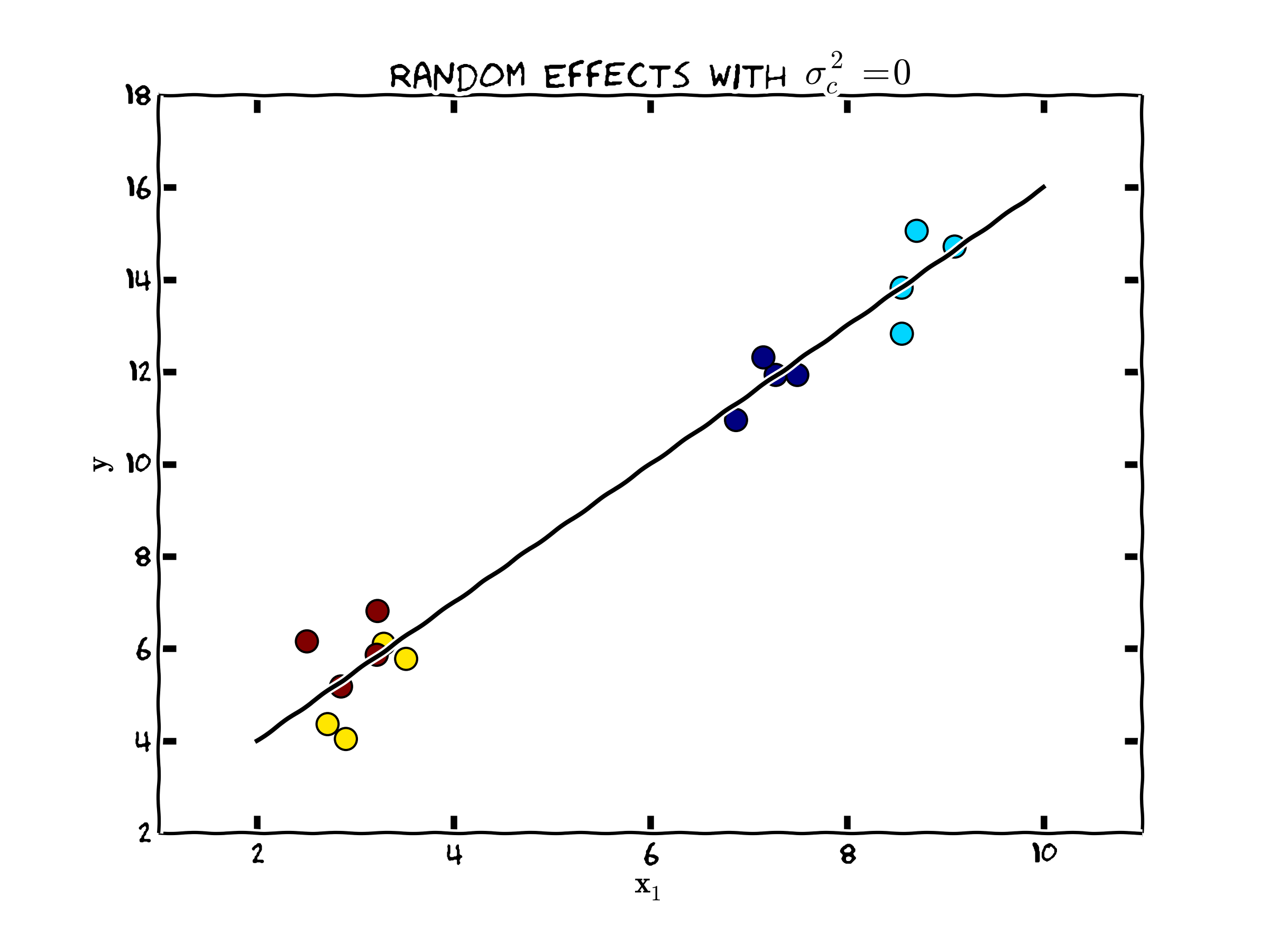
Figure 1. Random Effects when no Individual Heterogeneity
Since, \(E(c_i) = 0\), if the variance of \(c\) is zero, there is no individual specific heterogeneity since every \(c_i=0\). In this case, notice that \(\hat{\Omega}^{-1}\) collapses to
\[ \left(\begin{array}{cccc} \frac{ \hat{\sigma}^2_{\epsilon}}{{(\hat{\sigma}^2_{\epsilon}})^2 } & 0 & 0 & 0\\ 0 & \frac{ \hat{\sigma}^2_{\epsilon}}{{(\hat{\sigma}^2_{\epsilon}})^2 } & 0 & 0\\ 0 & 0 & \frac{ \hat{\sigma}^2_{\epsilon}}{{(\hat{\sigma}^2_{\epsilon}})^2 } & 0\\ 0 & 0 & 0 & \frac{ \hat{\sigma}^2_{\epsilon}}{{(\hat{\sigma}^2_{\epsilon}})^2 } \end{array}\right) = \frac{1}{\hat{\sigma}^2_{\epsilon}} \times I_{NT \times NT} \]
Consequently, the random effects estimator becomes
\begin{align} \mathbf{b}_{RE} &= \mathbf{(x' \hat{\Omega}^{-1} x)}^{-1}\mathbf{x' \hat{\Omega}^{-1} y} \nonumber \\ &= \mathbf{\left(x' \frac{1}{\hat{\sigma}^2_{\epsilon}} I x \right)}^{-1}\mathbf{x'} \frac{1}{\hat{\sigma}^2_{\epsilon}} \mathbf{Iy} \nonumber \\ &= \hat{\sigma}^2_{\epsilon}\mathbf{\left(x'x \right)}^{-1}\mathbf{x'} \frac{1}{\hat{\sigma}^2_{\epsilon}} \mathbf{y} \nonumber \\ &= \mathbf{\left(x'x \right)}^{-1}\mathbf{x'} \mathbf{y} \nonumber \\ &=\mathbf{b}_{OLS} \end{align}Thus, the pooled OLS estimator is the appropriate version of the random effects model, since there are no random effects. In this case, the weighted least squares estimator puts equal weight within individual observations and between individual observations.
-
Case 2: Individual heterogeneity dominates(\(\sigma^2_{c}\) is large relative to \(\sigma^2_{\epsilon}\))
As \(\sigma^2_c\) becomes larger, the weighted regression begins placing relatively more weight on the variation within individual observations in calculating \(\mathbf{b}_{RE}\). In the extreme case, we might consider the case where \(\sigma^2_{\epsilon}=0\). This would lead to the following graphical representation of the data. Note that the slope coefficient can be estimated completely within each set of individual observations. As more weight is placed on
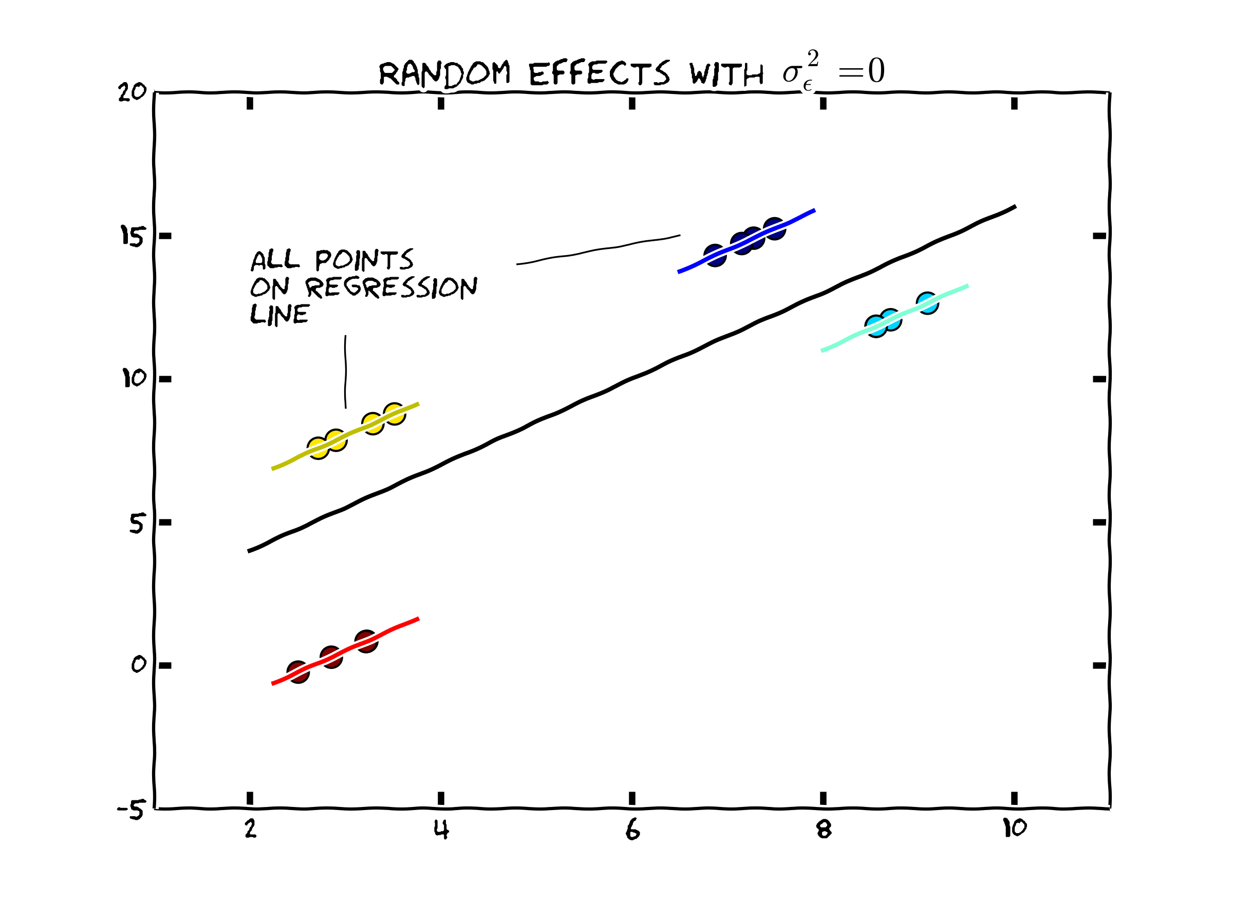
Figure 1. Random Effects when Individual Heterogeneity Dominates
In practice, however, there are fairly minor differences between the RE and OLS estimator. Consequently the test of OLS versus RE does not examine differences in parameter estimates since both are consistent.
Since the OLS model is nested within the RE model (by restricting \(\sigma^2_c = 0\)), we can use a maximum likelihood based test.
Inference
With that, we can calculate the parameter estimate given in equation \(\eqref{eq:re_estimator}\), having variance-covariance matrix
\begin{equation} \label{eq:re_varcov} Var(\mathbf{b}_{RE})=\left ( \mathbf{x}'\hat{\mathbf{\Omega}} \mathbf{x} \right )^{-1} \end{equation}One might also want to use robust standard errors if the model specification (including the structure assumed in \(\Omega\)) is incorrect. In this case, we can follow the methods and definition of \(\hat{\mathbf{V}}\) outlined in Section ([sec:olshet]) to write the robust random effects variance covariance estimator as
\begin{equation} \label{eq:re_robust_varcov} E[Var(\mathbf{b}_{RE})^{robust}]=\left ( \mathbf{x}' \hat{\mathbf{\Omega}} \mathbf{x} \right )^{-1}\left ( \mathbf{x}'\hat{\mathbf{\Omega}}^{-1} \hat{\mathbf{V}} \hat{\mathbf{\Omega}} \mathbf{x} \right )^{-1}\left ( \mathbf{x}' \hat{\mathbf{\Omega}} \mathbf{x} \right )^{-1} \end{equation}Another Estimation Method
The classic random effects model presented above places quite stringent restrictions on the error structure by way of the random effects definition of \(\Omega\). Further each and every realization of \(c_{i}\) is assumed to impart the identical covariance structure in the errors. It may well be the case that there is serial correlation among the individual specific errors that the random effects specification above ignores. Feasible Generalized Least Squares does not rely on \(\Omega\), but rather gets full information about how the random effects influence the error structure by way of the estimated errors from the pooled OLS regression shown in equation \(\eqref{eq:pooled_resids}\), and the calculation of \(\hat{v}\). Specifically, define
\begin{aligned} \label{eq:omega_fgls} \mathbf{\hat{\Omega}}_F=&\frac{1}{N}\sum^N_{i=1}\hat{\mathbf{v}_i}\hat{\mathbf{v}_i}' \\ =&\frac{1}{N} \left [ \begin{bmatrix} \hat{v}_{11}\hat{v}_{11} & \hat{v}_{11}\hat{v}_{12} & \ldots & \hat{v}_{11}\hat{v}_{1T} \\ \hat{v}_{12}\hat{v}_{11} & \hat{v}_{12}\hat{v}_{12} & \ldots & \hat{v}_{12}\hat{v}_{1T} \\ \vdots & \vdots & \ddots & \vdots \\ \hat{v}_{1T}\hat{v}_{11} & \hat{v}_{1T}\hat{v}_{12} & \ldots & \hat{v}_{1T}\hat{v}_{1T} \end{bmatrix} + \ldots + \begin{bmatrix} \hat{v}_{N1}\hat{v}_{N1} & \hat{v}_{N1}\hat{v}_{N2} & \ldots & \hat{v}_{N1}\hat{v}_{NT} \\ \hat{v}_{N2}\hat{v}_{N1} & \hat{v}_{N2}\hat{v}_{N2} & \ldots & \hat{v}_{N2}\hat{v}_{NT} \\ \vdots & \vdots & \ddots & \vdots \\ \hat{v}_{NT}\hat{v}_{N1} & \hat{v}_{NT}\hat{v}_{N2} & \ldots & \hat{v}_{NT}\hat{v}_{NT} \end{bmatrix} \right] \end{aligned}where the subscript on \(\hat{v}_{it}\) denotes individual \(i\) and time period \(t\). Finally, calculate the parameter estimates using
\begin{equation} \label{eq:fgls_estimator} \mathbf{b_{FGLS}}=\mathbf{(x' \hat{\Omega}_F^{-1} x)}^{-1}\mathbf{x' \hat{\Omega}_F^{-1} y} \end{equation}The variance-covariance matrix of the parameters is
\[Var(\mathbf{b}_{FGLS})=\mathbf{(x'x)^{-1}(x'\hat{\Omega}_Fx)(x'x)^{-1}}\]
So why not always use the FGLS estimator? It is more efficient since it extracts more information about the underlying process from the data? However, if \(N\) is not more than several times larger than T, than an unrestricted FGLS (where we allow for a richer variance covariance matrix for the error structure) can have poor finite sample properties since because we need to estimate \(T(T+1)/2\) elements. Conversely, random effects only requires the estimation of 2 elements describing the variance/covariance structure of the error.
Advantages of Random Effects Method
So long as the exogeneity assumptions are met (perhaps a big if), the biggest advantage of the random versus fixed effects approach is that one can include time invariant independent variables in \(\mathbf{x}\) [3]. For example, suppose that gun control laws differed across states but were constant for a 10 year period for which you have data. The Random Effects Model allows for consistent and efficient estimate of \(\beta\) and allows you to identify the effect of the gun control laws by exploiting the variation of these laws across states. The fixed effects model which we turn to next can not identify the effects of time invariant independent variables.
Implementation in R and Stata
The companion to this chapter shows how to implement many of these ideas in R and Stata.
[1] Although the differencing approach for T=2 is identical to the more sophisticated methods we will explore in the next chapter
[2] Another point to note is that any \(\hat{v}_{it}\hat{v}_{it+1}\) is not assured to be zero. In extreme cases, the average obtained in equation \(\eqref{eq:var_c}\) might be negative which is not suitable for a variance estimate (which must be positive) and is a sign that the Random Effects estimator is not suitable or that there is autocorrelation in \(\epsilon\). Wooldridge suggests including time dummies and perhaps searching for other models if this happens. Note: Stata will report \(\sqrt(\sigma^2_c)\) (which Stata calls ``sigma\u'') of zero if the average using the above equation is less than or equal to zero.
[3] Pooled OLS also has this advantage.