ECON 407: Fixed Effects for Panel Data
This page has been moved to https://econ.pages.code.wm.edu/407/notes/docs/index.html and is no longer being maintained here.
Use the same setup as in our other panel chapters, with the linear model
\begin{equation} \label{eq:fe_base} Y_{it}=\mathbf{X}_{it}\beta+c_i +\epsilon_{it} \end{equation}where \(X_{it}\) is a \(1 \times K\) vector of independent variables. Here we make our “usual assumptions”:
Assumption 1: \(E[\epsilon_{it}|X_{i1},\ldots,X_{iT},c_i]=0\)
Assumption 2: \(E[\epsilon_i\epsilon'_i]=\sigma^2 I_T\)
In the Random Effects model, we made a strong assumptions about the correlation between \(corr(c_i,X_i)=0\) to cleanse the model of the individual unobserved heterogeneity by putting the effect in the error term and correcting the error structure accordingly. In the fixed effects model, we make no such assumption about the correlation \(corr(c_i,X_i)=0\). The Fixed Effects Model deals with the \(c_i\) directly. We will explore several practical ways of estimating unbiased \(\beta\)'s in this context.
To see how truly wrong things can go, consider the following figure. In this case, \(c_i\) and the independent variable \(\mathbf{x}_i\) is highly positively correlated. The true relationship is quite different than what one would obtain via ordinary least squares or random effects. In fact, the OLS estimate of this data is highly significant (p<.0001) but of the wrong sign!
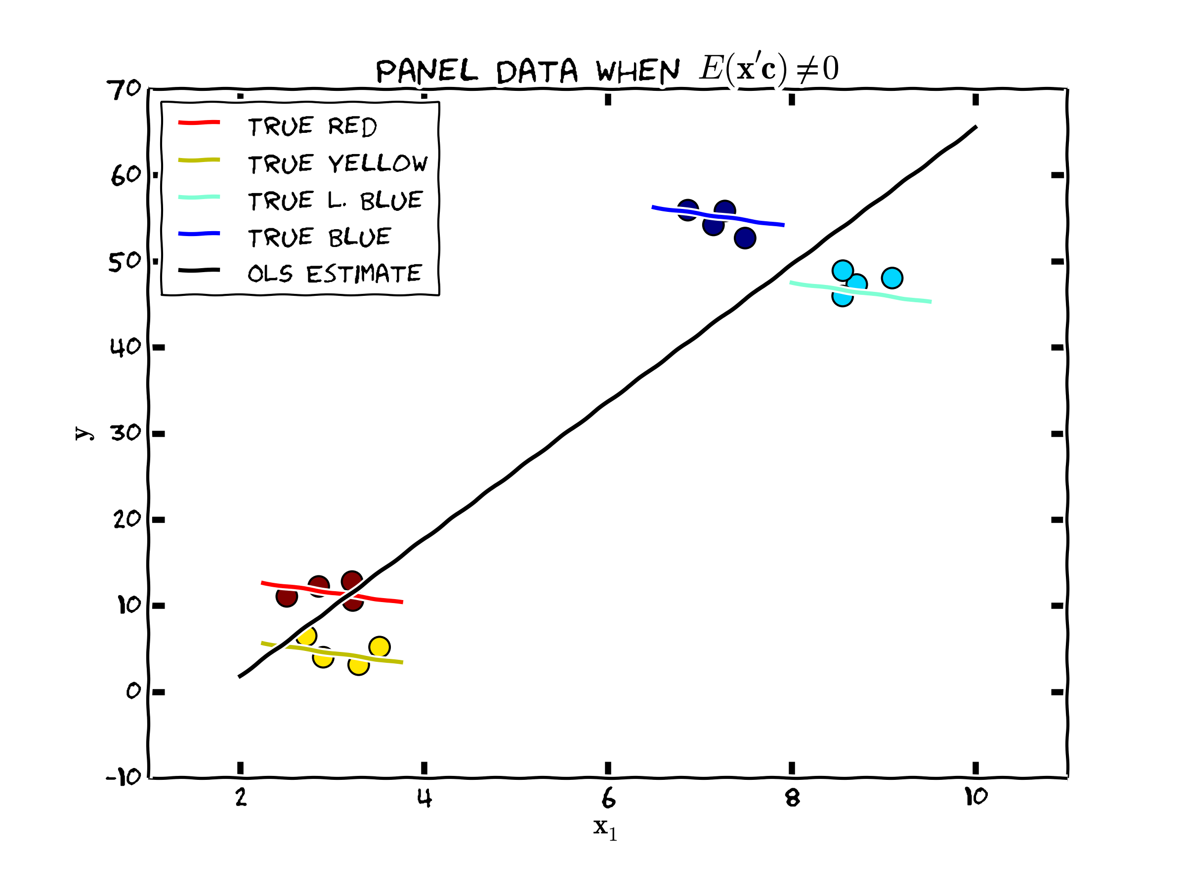
Figure 1. Unobserved Individual Heterogeneity and the Population Regression
The Dummy Variable Estimator
First consider estimating the \(c_i\) directly. Add an \(NT \times N-1\) dimensional time invariant vector, called Z to the regression model, where Z looks like this for observation \(i\)
\begin{equation} \mathbf{Z}_i=\begin{bmatrix} 0 & \cdots & 1 & \cdots & 0 \\ \vdots & & \vdots & & \vdots \\ 0 & \cdots & 1 & \cdots & 0 \\ \vdots & & \vdots & & \vdots \\ 0 & \cdots & 1 & \cdots & 0 \end{bmatrix}_{T \times (N-1)} \end{equation}In general, this vector will have elements \(Z_{it,j}=1\) when \(i=j\) and 0 otherwise. We construct this for each cross section unit, \(N\) and denote the vector as \(Z_i\) for each individual \(i\). Basically, we are estimating a dummy variable for each cross sectional unit in the analysis. That is, we are going to use these dummy variables to estimate the fixed effects directly. We term this approach the “Dummy Variable Approach”. Using this approach, we can write the estimating equation as
\[\mathbf{Y_{it}=X_{it}\beta+Z_{it} c +\epsilon_{it}}\]
where c is an \(N \times 1\) vector of individual fixed effects. Deriving the least squares estimator for \(\beta\) in this case,
\[\underset{\mathbf{c,b}}{min}S(\mathbf{b})=\left(\mathbf{Y-X b-Z c} \right )'\left(\mathbf{Y-X b-Z c} \right )\]
is just the OLS estimator for \(b\) and \(c\). The estimators are unbiased, but the estimates for \(c\) is not consistent. Think about getting more cross section units (more \(N\)), we don't get more information about \(c_i\). Consider the special case of a regression where there are no independent variables in \(\mathbf{X_{it}}\). In that case,
\[\hat{c}_i=\sum^{T}_{t=1}{\frac{Y_{it}}{T}}\]
having variance \(\frac{\sigma^2}{T}\) which does not go zero as \(N\) goes to infinity. Refer to this estimator the dummy variable estimator \(\mathbf{b}_{dv}\). The variance of \(\epsilon\), \(\sigma_{\epsilon}^2\) is
\[\frac{1}{NT-K-N-1}\hat{\mathbf{\epsilon_{dv}}}'\hat{\mathbf{\epsilon_{dv}}}\]
where
\[\mathbf{\hat{\epsilon}_{dv}}=\left(\mathbf{Y-X b -Z c} \right )\]
Besides the consistency problem, this estimator requires the identification of \(N+K-1\) parameters which depending on how many cross sectional units there are may be computationally challenging, since it requires inverting an \((N+K) \times (N+K)\) dimension matrix.
The Demeaning Estimator
To overcome these difficulties, the remaining approaches attempt to adjust the estimator for the presence of individual unobserved effects without estimating them directly, yet unlike random effects they do not simply put the effect in the model error term and make strong assumptions about correlations. Consider the “within” means, the means of \(X\) and \(Y\) for each cross sectional unit
\[\bar{Y_i}=\frac{1}{T}\sum^T_{t=1}Y_{it} \hspace{.2in}and\hspace{.2in} \bar{X_i}=\frac{1}{T}\sum^T_{t=1}X_{it}\]
and writing the deviations from the means for X and Y as
\[\ddot{Y}_{it}=Y_{it}-\bar{Y_i} \hspace{.2in}and\hspace{.2in} \ddot{X}_{it}=X_{it}-\bar{X_i}\]
Note that it is possible to write this in linear algebra form for each cross sectional unit N. Defining \(A=I_t-\frac{\imath_T \imath'_T}{T}\), write
\[\ddot{X_i}=AX_i\]
Note, we need to define \(\imath_T\) as a \(T\times 1\) column of 1's, so that \(\imath_T\imath'_T\) is a \(T \times T\) matrix whose elements are all equal to 1. We can recover the demeaning estimator (\(b_{d}\)) for \(\beta\) by OLS on the demeaned data as
\[\mathbf{b_d=(\ddot{X}'\ddot{X})^{-1}\ddot{X}'\ddot{Y}}\]
It is possible to show that \(\mathbf{b_d=b_{dv}}\), but note that this regression does not estimate the vector \(\mathbf{c}\). Wooldridge calls this the fixed effects estimator, and this is probably what most statistical packages do when you ask for a fixed effects estimator and is sometimes called the “within” estimator.[1]
While the regression estimates are unbiased, since \(E(\ddot{\mathbf{\epsilon}}|\mathbf{X}_i)=0\), the standard variance covariance matrix from simple OLS is not correct. To see this, recall that
\begin{aligned} E[\ddot{\epsilon}^2_{it}]=&E[\mathbf{(\epsilon_{it}-\bar{\epsilon_i})^2}]=E[\epsilon_{it}^2-2\epsilon_{it}\bar{\epsilon_i}-\bar{\epsilon_i}^2]\\ =&\sigma_{\epsilon}^2-2\sigma_{\epsilon}^2/T+\sigma_{\epsilon}^2/T \end{aligned}Finally giving
\begin{equation} \label{eq:var_dm} Var(\ddot{\epsilon}^2_{it}) = E[\ddot{\epsilon}^2_{it}] =\sigma_{\epsilon}^2(1-1/T) \end{equation}For covariances, we have
\begin{aligned} E[\ddot{\epsilon}_{it}\ddot{\epsilon}_{is}]=&E[(\epsilon_{it}-\bar{\epsilon_{i}})(\epsilon_{is}-\bar{\epsilon_{i}})]\\ =&0-\sigma_{\epsilon}^2/T-\sigma_{\epsilon}^2/2 +\sigma_{\epsilon}^2/T\\ =&-\sigma_{\epsilon}^2/T \end{aligned}We need to be mindful of these results for adjusting the variance-covariance matrix of our estimated parameters before we can perform statistical inference.
Following similar steps as in the OLS chapter, the variance of our estimator \(\mathbf{b}_d\) is
\begin{aligned} Var(\mathbf{b_d}|x)=&E[(b_d-b)(b_d-b)'|x]\\ =&E[(\ddot{X}'\ddot{X})^{-1}\ddot{X}'\ddot{Y}-\beta)(\ddot{X}'\ddot{X})^{-1}\ddot{X}'\ddot{Y}-\beta)'] \\ =&E[(\ddot{X}'\ddot{X})^{-1}\ddot{X}'(\ddot{X}\beta+\epsilon)-\beta)(\ddot{X}'\ddot{X})^{-1}\ddot{X}'(\ddot{X}\beta+\epsilon)-\beta)'] \\ =&\sigma_{\epsilon}^2 E[(\ddot{X}'\ddot{X})^{-1}] \end{aligned}So note, we are mixing demeaned data and information from the "un" demeaned errors for deriving the variance covariance matrix of our estimates.
We can use equation \eqref{eq:var_dm} to obtain an empirical estimate of \(\sigma_{\epsilon}^{2}\) from the demeaned predicted residuals \(\ddot{\epsilon}_{it}\). This is very useful, since to recover un-demeaned predicted errors, we would need estimates for all of the unobserved heterogeneity terms \(\hat{c}_i\) which we don't have nor can we estimate consistently for small \(T\). So the estimate for \(\sigma^2_\epsilon\) can be calculated as \[\hat{\sigma}^2_\epsilon=\frac{(\ddot{Y}-\ddot{X}\beta)'(\ddot{Y}-\ddot{X}\beta)}{N(T-1)-K}\]
The First Differences Estimator
You have already seen how to estimate the first differences model from the introduction to panel data methods. The model can be extended to \(T>2\) in a trivial way. We present it here again for completeness.
Suppose that for each individual, we have a panel of two periods (\(t=1,2\)). Perhaps we could apply a differencing approach for each individual i to rid the model of \(c_i\), since
\begin{aligned} \Delta y_{i} = & \beta \left (x_{i2}-x_{i1} \right ) + \left (c_i-c_i \right) + \left (\epsilon_{i2}-\epsilon_{i1} \right) \\ = & \Delta x_{i} \beta + \Delta \epsilon_{i} \end{aligned}since the individual-specific effect is time invariant, these constants drop from the model, and we are still left with our parameters of interest (\(\beta\)). So in a panel with two time periods, we are left with one standard cross section equation consisting of individual level data denoted by
\[\Delta y = \Delta x \beta + \Delta \epsilon\]
where
\[\Delta y = \begin{bmatrix} \Delta y_1 \\ \vdots \\ \Delta y_i \\ \vdots \\ \Delta y_N \end{bmatrix}\]
and \(\Delta x\) is defined in a similar fashion. Will a simple OLS estimate of this cross section be unbiased and consistent?
The orthogonality condition is the first place to start with answering this question. Recall that in a standard regression model of the previous chapter, the proof of unbiasedness rests with the OLS orthogonality assumption, and invoking the fact that \(E(x'\epsilon)=0\) allows us to show that \(E(b)=\beta\). For OLS to be unbiased, we need a similar condition here. Note that this means
\begin{equation} E(\Delta x' \Delta \epsilon)=0 \label{eq:first_diff_assumption1} \end{equation}and the following inverse must exist
\begin{equation} \label{eq:first_diff_assumption2} (\Delta x' \Delta x)^{-1} \end{equation}requiring that \(\Delta x\) must be of full rank.
What are the implications of these assumptions? First consider Equation \(\eqref{eq:first_diff_assumption1}\). This condition can be rewritten as
\begin{aligned} & E \left [(x_{2}-x_{1})'(\epsilon_{2}-\epsilon_{1}) \right]=0 \\ & E \left [(x_{2}'\epsilon_{2}+x_{1}'\epsilon_{1}-x_{1}'\epsilon_{2}-x_{2}'\epsilon_{1}) \right]=0 \end{aligned}The first two terms are zero by definition given the assumption \(E(x'\epsilon)=0\). Note however, that in this framework, we also need to assume
\begin{aligned} E(x_{1}'\epsilon_{2})&=0 \\ E(x_{2}'\epsilon_{1})&=0 \end{aligned}these highlight the even more restrictive orthogonality conditions we need to assume to implement this type of approach (known as Strict Exogeneity).
It is also useful to think carefully about equation \(\eqref{eq:first_diff_assumption2}\). Since the matrix \(\Delta x\) is comprised of elements differenced across two periods, x may not contain any variable that is constant across time for every person in the sample. For example, if the Kth element of x were to contain a dummy variable equal 1 if a person's sex is female and 0 if male, then
\[\Delta x_K= \begin{bmatrix} \color{blue}{1-1} \\ \color{blue}{\vdots} \\ \color{blue}{1-1} \\ \vdots \\ \color{red}{0-0} \\ \color{red}{\vdots} \\ \color{red}{0-0} \\ \vdots \\ \color{green}{1-1} \\ \color{green}{\vdots} \\ \color{green}{1-1} \\ \end{bmatrix}\]
so the matrix \(\Delta x\) would not be of full rank since every element in column K is equal to zero. For some of the panel data models we will consider (i.e. the Fixed Effects Model), your independent variables must vary across periods in your panel. This is very important to remember.
Which Fixed Effects Estimator to Use?
It should be noted that if \(T=2\), all of the results presented here give exactly equivalent results for the estimated parameters and variance/covariance matrices. Since first differences is easy to implement and does not require the estimation of the N constants capturing unobserved heterogeneity, it is probably the way to proceed. If \(T>2\), then the choice of estimator depends on the assumptions one makes about the errors, \(\epsilon_{it}\). If these errors are serially uncorrelated, then the Dummy Variable Estimator is preferred whereas if the error follows a random walk the First Differences Estimator is preferred. If any of the usual standard endogeneity problems are thought to be present: measurement error, time varying ommitted variables, and simultaneity, then we have problems and our estimates are not consistent.
Testing for Endogeneity in a Fixed Effects Setting
Endogeneity Testing proceeds in a very similar manner as in the endogeneity chapter. Here are the steps:
- Partition your matrix of explanatory variable for each individual as \(\mathbf{x_i}=\left[ \mathbf{x_{i1} \hspace{.15in} x_{i2}}\right]\). Note that \(\mathbf{x}_{i1}\) is the subset of exogenous independent variables and \(x_{i2}\) is the the potentially endogenous explanatory variable having an instrument \(z_{i2}\).
-
From the relevancy equation, run the regression
\begin{equation} \Delta {x_{i2t}}=\Delta \mathbf{x}_{i1t} \mathbf{a} + \Delta \mathbf{z}_{i2t} b + \Delta r_{it} \end{equation}and recover \(\Delta \hat{r}_{it}\)
-
As in the endogeneity chapter,
\begin{equation} \Delta y_{it}=\Delta \mathbf{x}_{it} \beta + \Delta \hat{r}_{it} \delta +\psi \end{equation}And test for \(H_0: \delta=0\). Rejecting \(H_0\) is a strong signal of an endogeneity problem.
If we reject the null hypothesis, then we can apply a panel version of IV Regression (this will briefly be demonstrated in class).
Testing for Random versus Fixed Effects
The critical difference between the random and fixed effects approaches is whether \(c_i\) is correlated with \(\mathbf{x}_{it}\). If it is, then the random effects approach, which simply puts \(c_i\) in the error term will lead to biased estimates relative to the fixed effects estimator. As in the Chapter on endogeneity, we need to test to see how "different" the two estimated \(\beta\) vectors are and to do this, we use the Hausman test.
Letting \(\hat{\delta}_{RE}\) and \(\hat{\delta}_{FE}\) represent the regression results obtained using only the time varying elements of \(\mathbf{x}\), the Hausman statistic is
\[H=(\hat{\delta}_{FE}-\hat{\delta}_{RE})'\left[\hat{VAR}_{FE}-\hat{VAR}_{RE} \right]^{-1}(\hat{\delta}_{FE}-\hat{\delta}_{RE})\]
is distributed with \(\chi^2_M\) degrees of freedom where M are the number of parameters estimated in each model. Rejecting the NULL hypothesis, that the unobserved individual effects are uncorrelated with the independent variables in the model. A failure to reject the NULL hypothesis provides a basis for choosing the more "restrictive" random effects approach.
Implementation in R and Stata
The companion to this chapter shows how to implement many of these ideas in R and Stata.
[1] The "between" estimator uses only variation between cross section units. It is recovered by the regression \(\bar{Y}_i=\bar{X}_i \beta +c_i+u_i\), or the average of Equation \eqref{eq:fe_base}.