The Heckman Sample Selection Model

This page has been moved to https://econ.pages.code.wm.edu/407/notes/docs/index.html and is no longer being maintained here.

We are interested in estimating the model

\begin{equation} \mathbf{y^*=xb + \epsilon} \end{equation}

but for a subset of our data, the dependent variable is either missing or coded to some arbitrary values (e.g. 0 or -999). Of concern however, is that the pattern of this missingness is non-random in a way that could induce bias in our estimated $\beta$'s if we apply OLS to observed values from the above equation.

Selection Mechanism

Suppose that the pattern of missingness (I'll refer to this as censored hereafter) is related to the latent (unobserved) process

\begin{equation} \mathbf{z}^* = \mathbf{w}\gamma + \mathbf{u} \end{equation}

From this process, the researcher can observe

\begin{align} z_i =& 1 \text{ if } z^*_i > 0 \\ =&0 \text{ if } z^*_i \le 0 \end{align}

or $z_i=1$ ($y_i$ not censored) when

\begin{equation} u_i \ge - \mathbf{w}_i\gamma \end{equation}

The probability of $y_i$ not censored is

\begin{align} Pr(u_i \ge - \mathbf{w}_i\gamma) =& 1- \Phi(-\mathbf{w}_i\gamma)\\ &=\Phi(\mathbf{w}_i\gamma) \end{align}

if we are willing to assume that $\mathbf{u}\sim N(\mathbf{0},\mathbf{I})$. Note for identification purposes in the Heckman Model we restrict $Var(u_i) = 1$. Also note that $1- \Phi(-\mathbf{w}_i\gamma)=\Phi(\mathbf{w}_i\gamma)$ by symmetry of the standard normal distribution.

To visualize this, consider the following figure. The probability of $y_i$ not being censored ($Pr(u_i \ge - \mathbf{w}_i\gamma)$) is the set of errors greater than $-\mathbf{w}_i\gamma$. The probability that an error draw satisfies this condition is the darker shaded area to the right of $-\mathbf{w}_i\gamma$.

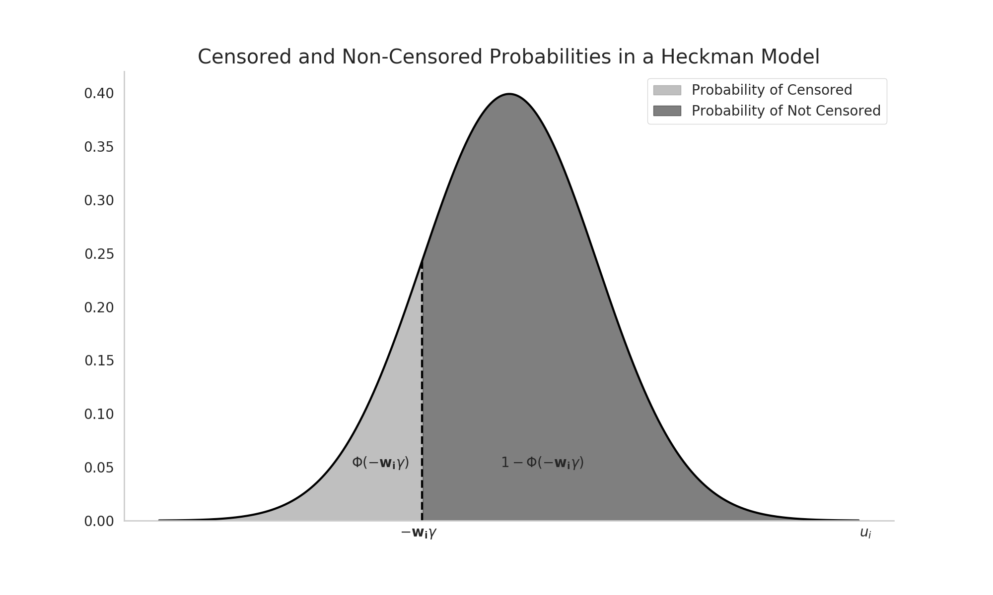
Figure 1: Probabilities in the Selection Mechanism in a Heckman Model

Amounts Mechanism and Sample Selection Bias

Having constructed a model a model for censoring, we can construct "amounts" equation as follows. Denoting $\mathbf{y}$ as the not censored (observed) dependent variable, the censoring model defines what is in the estimation sample as

\begin{align} y_i = y^*_i = \mathbf{x}_i \beta + \epsilon_i \text{ observed, if $z_i$ = 1} \end{align}

Finally, the joint distribution of the errors in the selection ($u_i$) and amounts equation ($\epsilon$) is distributed iid as

\begin{equation} \begin{bmatrix} u_i \\ \epsilon_i \end{bmatrix} \sim Normal\left( \begin{bmatrix} 0 \\ 0 \end{bmatrix}, \begin{bmatrix} 1 & \rho \\ \rho & \sigma^2_\epsilon \end{bmatrix} \right) \end{equation}

To see how the selection and amounts model are related, consider

\begin{align} E(y_i | y_i \text{ observed}) = & E(y_i | z^* > 0 ) \\ =&E(y_i | u_i > -\mathbf{w}_i \gamma) \\ =&\mathbf{x}_i \beta + E(\epsilon_i | u_i > -\mathbf{w}_i \gamma) \\ =&\mathbf{x}_i \beta + \rho \sigma_\epsilon \frac{\phi(\mathbf{w}_i \gamma)}{\Phi(\mathbf{w}_i \gamma)} \end{align}

What is immediately apparent is that the conditional mean ($E(y_i | y_i \text{ observed})$) differs from the unconditional mean ($\mathbf{x}_i\beta$) only if $\rho \neq 0$ since all the other elements in the far right hand term (i.e., the variance of the error in the amounts equation, $\sigma_\epsilon$, and the Inverse Mills Ratio, $\frac{\phi(\mathbf{w}_i \gamma)}{\Phi(\mathbf{w}_i \gamma)}$) in the preceding equation are strictly positive. So if the errors in the amounts and selection equations are uncorrelated ($\rho=0$) we can safely apply ordinary least squares to uncover unbiased estimates for $\beta$ and can ignore endogenous selection effects and the selection equation portion of the model.

However, there are some further nuances to consider. Denoting the correlation amongst the two sets of independent variables in the model $\mathbf{x},\mathbf{w}$ as $\rho_{\mathbf{x},\mathbf{w}}$, we examine the following four cases of correlation patterns amongst data and errors. As the final equation above shows, when $\rho$ is zero (Cases 1 and 2) in the Table below, OLS will always give unbiased $\beta$ even if $\rho_{\mathbf{x},\mathbf{w}}$ is non-zero. This is happening because the missingness patterns in $\mathbf{y}$ are essentially random or select cases in ways that are symmetric around the regression line that preserves slope and intercept coefficients (we have plots of these cases later for providing more intuition about this statement).

Table 1: Visualizing Sample Selection Bias for Data and Error Correlations

Case 1	$\rho=0$	$\rho_{\mathbf{x},\mathbf{w}}=0$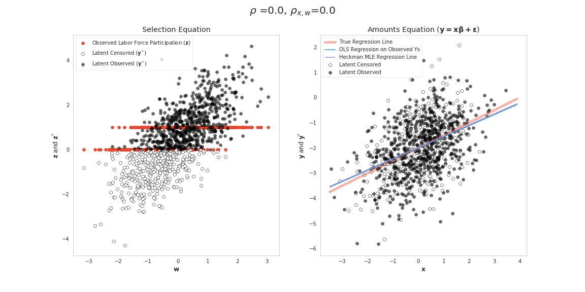
Case 2	$\rho=0$	$\rho_{\mathbf{x},\mathbf{w}}\neq 0$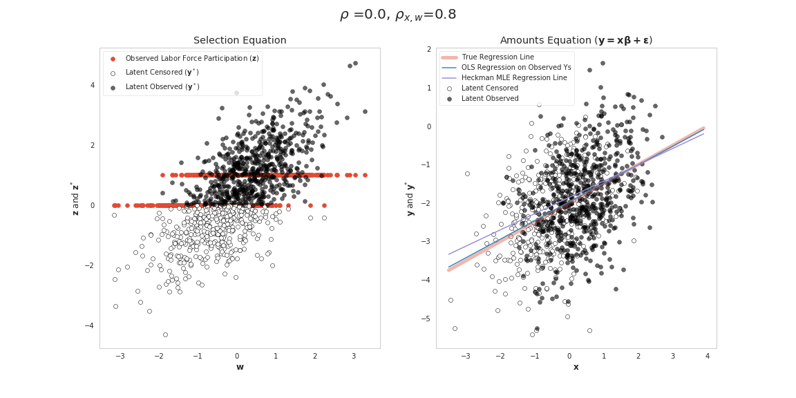
Case 3	$\rho\neq 0$	$\rho_{\mathbf{x},\mathbf{w}}=0$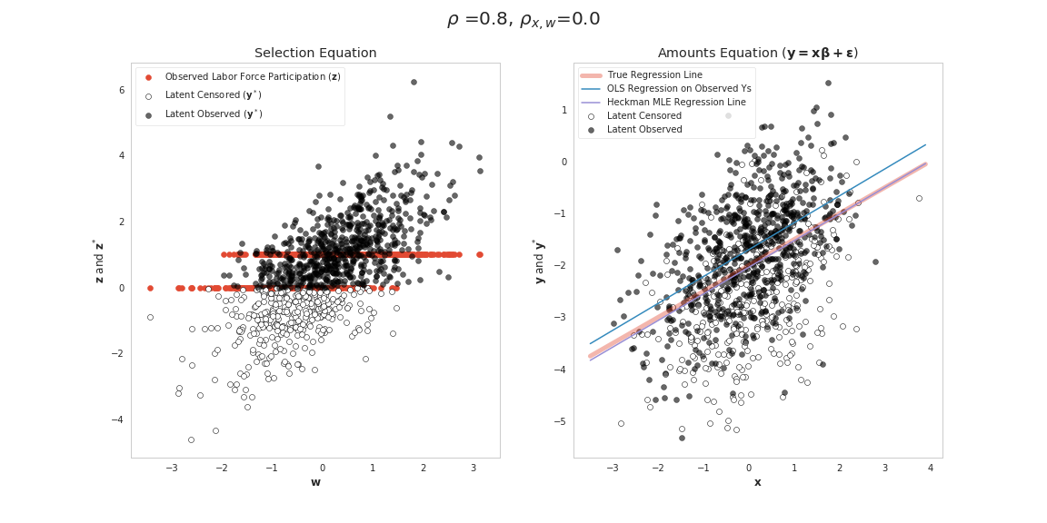
Case 4	$\rho\neq 0$	$\rho_{\mathbf{x},\mathbf{w}}\neq 0$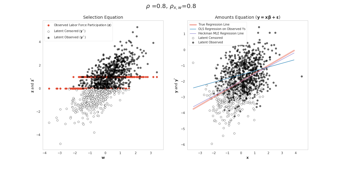

Cases 3 and 4 are more interesting and represent instances where OLS will be inconsistent and we should apply the Heckman Model. For gaining intuition about how cases 3 and 4 differ consider again the conditional mean

\begin{equation} E(y_i | y_i \text{ observed}) = \mathbf{x}_i \beta + \rho \sigma_\epsilon \frac{\phi(\mathbf{w}_i \gamma)}{\Phi(\mathbf{w}_i \gamma)} \end{equation}

We can think of the preceding equation as guiding the regression equation we ought to be estimating if the sample selection process as outlined above is happening. If instead, we ignore the final term ($\rho \sigma_\epsilon \frac{\phi(\mathbf{w}_i \gamma)}{\Phi(\mathbf{w}_i \gamma)}$) when in fact $\rho\neq 0$ then we are putting this information into the error term of the misppecified OLS model regressing $\mathbf{y}$ on $\mathbf{x}$ making the estimation equation

\begin{equation} \mathbf{y = x \tilde{\beta} + \psi} \end{equation}

where $\psi = \rho \sigma_\epsilon \mathbf{IMR} + \epsilon$, where $\mathbf{IMR}$ is the $N \times 1$ vector

\begin{equation} \begin{bmatrix} \frac{\phi(\mathbf{w}_1 \gamma)}{\Phi(\mathbf{w}_1 \gamma)}\\ \vdots \\ \frac{\phi(\mathbf{w}_i \gamma)}{\Phi(\mathbf{w}_i \gamma)} \\ \vdots \\ \frac{\phi(\mathbf{w}_N \gamma)}{\Phi(\mathbf{w}_N \gamma)} \end{bmatrix} \end{equation}

For the OLS estimator to be unbiased in this context, we need $E[\mathbf{b}] = \beta$, so that (without showing steps in proof which is analogous to the OLS proof of unbiasedness):

\begin{align} E[\mathbf{b}] =& \beta +E[(\mathbf{x'x})^{-1}\rho \sigma_\epsilon \mathbf{x}'\mathbf{IMR} + (\mathbf{x'x})^{-1}\mathbf{x}'\epsilon] \\ =& \beta + \rho \sigma (\mathbf{x'x})^{-1}E[\mathbf{x}'\mathbf{IMR}] \end{align}

since $E[\mathbf{x}'\epsilon]=0$ and $\rho$ and $\sigma_\epsilon$ are unknown constants. If $\rho \neq 0$, this term won't be zero. Simplifying the last term from above further, we have

\begin{align} \rho \sigma (\mathbf{x'x})^{-1}E[\mathbf{x}'\mathbf{IMR}] = \rho \sigma (\mathbf{x'x})^{-1}(\mathbf{x}'\mathbf{IMR} + Cov(\mathbf{x}',\mathbf{IMR})) \end{align}

For case 3, the independent variables in the model $\mathbf{x}$ and $\mathbf{w}$ are uncorrelated so it is likely that $Cov(\mathbf{x}',\mathbf{IMR})$ is very close to zero, since all variation in the relationship is being driven by the two sets of independent variables in the model ($\mathbf{x}$ and $\mathbf{w}$). Setting $Cov(\mathbf{x}',\mathbf{IMR})=0$, shows that there will still be bias since $\mathbf{x}'\mathbf{IMR}$ won't be zero. Here we are adding (or subtracting depending on the sign of $\rho$) a constant value to the model with mean $\rho \sigma (\mathbf{x'x})^{-1} \mathbf{x}'\mathbf{IMR}$. So this miss-specified model's constant term will need to depart from the true value $\beta_0$ to account for this positive or negative shift in the mean value of all observation's errors. However, since there is no correlation amongst $\mathbf{x}$ and $\mathbf{w}$ in our miss-specified OLS model we won't impart missing variable bias on our slope coefficients. The Figure for case 3 above shows this happening. Cases that are selected tend to have higher draws for $\epsilon$. So the points that are censored tend to be below (for our case here) in a way that would only affect the intercept coefficient.

For case 4, we have the bias imparted on our intercept coefficient as discussed above and bias induced by correlation between our model error $\psi$ and $\mathbf{x}$ (since $\mathbf{x}$ and $\mathbf{w}$ are correlated). This has the effect of also biasing our slope coefficients. The Figure for Case 4 shows how this is happening visually. As in Case 3, the observations that tend to be included in the amounts equation (the dark points in the right panel) on average tend to be above the True Regression line. This is happening because in the selection equation we tend select observations having higher draws of $u_i$. Since (for this example) $u_i$ and $\epsilon_i$ are positively correlated, we also tend to be selecting cases above the True regression line. Additionally, when $\mathbf{w}$ and $\mathbf{x}$ are correlated the cases we select tend to be (for this example) higher values of our independent variable $\mathbf{x}$ (since higher values of $\mathbf{z}$ tend to be selected). This has the effect of shifting the some of points that are censored (compared to Case 3) below the regression line which can lead to bias if we apply OLS.

Model Log-Likelihood

Defining person i's contribution to the log-likelihood function ($C_i$) as

\begin{equation} \small C_i = \left\{ \begin{aligned} &ln\Phi \left(\frac{\mathbf{w_i \gamma} + \rho \left (\frac{y_i - \mathbf{x}_i \beta}{\sigma_\epsilon}\right)} {\sqrt{1 - \rho^2}}\right) - \frac{1}{2} \left( \frac{y_i - \mathbf{x}_i\beta}{\sigma_{\epsilon}} \right)^2-ln\left(\sigma_{\epsilon}\sqrt{2\pi}\right) \text{, $z_i$ = 1}\\ &ln\left( 1 - \Phi(\mathbf{w}_i\gamma) \right) \text{, $z_i$ = 0} \end{aligned} \right. \end{equation}

The log-likelihood function is

\begin{equation} LogL = \sum_{i = 1}^N C_i \end{equation}

Source: Stata pdf manual for Heckman Model.

Estimation

There are two estimators one can employ. The first method (known as the two-step method) was the only practical way to estimate the model when the paper was first published in 1979. This method follows these steps:

Run Probit on the Selection Model
Recover Estimated Inverse Mills Ratio
Using Odinary Least Squares, run the regression
\begin{equation} y_i = \mathbf{x}_i \beta + \rho \sigma_\epsilon \frac{\phi(\mathbf{w}_i \hat{\gamma})}{\Phi(\mathbf{w}_i \hat{\gamma})} \end{equation}
where $\rho \sigma_\epsilon$ is treated as a single parameter to be estimated.
"Back Out" separate estimates for $\rho$ and $\sigma_\epsilon$
Adjust standard errors to account for the fact that the Inverse Mills Ratio is an estimate (and hence random) covariate in the above model.

The key two steps are to first run a probit and using information from the results from that model estimate a corrected form of the OLS model. This is the only estimation method available in a beta branch of Python Statsmodels as of November 2018.

The second and preferred method is to use Maximum Likelihood over the full parameter set $\beta, \gamma, \rho$, and $\sigma$ in the log-likelihood function above. This is the default method in Stata.

Notes

The python code generating the toy data for the figures above is given below. This version examines Case 4.

import numpy as np
import pandas as pd

# true parameters
rho_t = np.array([0.8])
rho_x_w_t = np.array([0.8])
gamma_t = np.array([.5,1.0])
beta_t = np.array([-2.0,0.5])
sigma_e_t = np.array([1.0])
N =5000

# generate toy data consistent with heckman:
# generate potentially correlated x,w data
mean_x_w = np.array([0,0])
cov_x_w = np.array([[1,rho_x_w_t[0]],[rho_x_w_t[0], 1]])
w, x = np.random.multivariate_normal(mean_x_w, cov_x_w, N).T

# add constant to first position and convert to DataFrame
w_ = pd.DataFrame(np.c_[np.ones(N),w],columns=['Constant (Selection)','Slope (Selection)'])
x_ = pd.DataFrame(np.c_[np.ones(N),x], columns=['Constant','Slope'])

# generate errors 
mean_u_eps = np.array([0,0])
cov_u_eps = np.array([[1,rho_t[0]],[rho_t[0],sigma_e_t]])
u, epsilon = np.random.multivariate_normal(mean_u_eps, cov_u_eps, N).T

# generate latent zstar
zstar = w_.dot(gamma_t) + u
# generate observed z (indicator=1 if zstar is positive)
z = zstar > 0  

# generate latent ystar
ystar = x_.dot(beta_t) + epsilon
y=ystar.copy()
# generate observed y [if z=0, set y to NaN]
y[~z] = np.nan

stata_data = pd.DataFrame(np.c_[y,z,x,w], columns=['y','z','x','w'])
stata_data.to_stata('/tmp/heckman_data.dta')
print(stata_data.head())

          y    z         x         w
0 -0.361568  1.0  1.611681  1.246033
1  0.286073  1.0  0.533292  1.275710
2 -1.923910  1.0 -0.925883 -0.132921
3       NaN  0.0  0.415372 -0.302027
4       NaN  0.0  0.564962 -0.472421

We can estimate a Two-Step Heckman Model in Python using an unmerged branch from StatsModels (this replicates the Stata two-step results).

import heckman as heckman
res = heckman.Heckman(y, x_, w_).fit(method='twostep')
print(res.summary())

       Heckman Regression Results      
=======================================
Dep. Variable:                        y
Model:                          Heckman
Method:                Heckman Two-Step
Date:                  Sun, 18 Nov 2018
Time:                          13:11:04
No. Total Obs.:                    5000
No. Censored Obs.:                 1825
No. Uncensored Obs.:               3175
==============================================================================
                 coef    std err          z      P>|z|      [0.025      0.975]
------------------------------------------------------------------------------
Constant      -1.9734      0.036    -54.832      0.000      -2.044      -1.903
Slope          0.4901      0.023     20.859      0.000       0.444       0.536
========================================================================================
                           coef    std err          z      P>|z|      [0.025      0.975]
----------------------------------------------------------------------------------------
Constant (Selection)     0.5010      0.022     23.084      0.000       0.458       0.544
Slope (Selection)        0.9800      0.028     35.171      0.000       0.925       1.035
================================================================================
                   coef    std err          z      P>|z|      [0.025      0.975]
--------------------------------------------------------------------------------
IMR (Lambda)     0.7474      0.061     12.179      0.000       0.627       0.868
=====================================
rho:                            0.771
sigma:                          0.970
=====================================

First table are the estimates for the regression (response) equation.
Second table are the estimates for the selection equation.
Third table is the estimate for the coef of the inverse Mills ratio (Heckman's Lambda).

And in Stata, we can estimate the Full Information Maximum Likelihood model over the toy dataset as

use /tmp/heckman_data
heckman y x, select(z=w)


Iteration 0:   log likelihood = -6344.3615
Iteration 1:   log likelihood =  -6343.826
Iteration 2:   log likelihood = -6343.8258

Heckman selection model                         Number of obs     =      5,000
(regression model with sample selection)              Selected    =      3,175
                                                      Nonselected =      1,825

                                                Wald chi2(1)      =     701.15
Log likelihood = -6343.826                      Prob > chi2       =     0.0000

------------------------------------------------------------------------------
             |      Coef.   Std. Err.      z    P>|z|     [95% Conf. Interval]
-------------+----------------------------------------------------------------
y            |
           x |   .4905715   .0185267    26.48   0.000     .4542598    .5268832
       _cons |  -1.987012   .0239226   -83.06   0.000    -2.033899   -1.940124
-------------+----------------------------------------------------------------
z            |
           w |   .9725891   .0267484    36.36   0.000     .9201633    1.025015
       _cons |   .5036102   .0214809    23.44   0.000     .4615085     .545712
-------------+----------------------------------------------------------------
     /athrho |   1.081067   .0626042    17.27   0.000     .9583655    1.203769
    /lnsigma |  -.0234431    .016779    -1.40   0.162    -.0563294    .0094431
-------------+----------------------------------------------------------------
         rho |   .7935946   .0231765                      .7435469    .8348007
       sigma |   .9768295   .0163902                      .9452277    1.009488
      lambda |   .7752066    .032709                      .7110981    .8393151
------------------------------------------------------------------------------
LR test of indep. eqns. (rho = 0):   chi2(1) =   216.27   Prob > chi2 = 0.0000


Case 1	\(\rho=0\)	\(\rho_{\mathbf{x},\mathbf{w}}=0\)
Case 2	\(\rho=0\)	\(\rho_{\mathbf{x},\mathbf{w}}\neq 0\)
Case 3	\(\rho\neq 0\)	\(\rho_{\mathbf{x},\mathbf{w}}=0\)
Case 4	\(\rho\neq 0\)	\(\rho_{\mathbf{x},\mathbf{w}}\neq 0\)