{
"cells": [
{
"cell_type": "markdown",
"metadata": {},
"source": [
"This page has been moved to [https://econ.pages.code.wm.edu/414/syllabus/docs/index.html](https://econ.pages.code.wm.edu/407/notes/docs/index.html) and is no longer being maintained here."
]
},
{
"cell_type": "markdown",
"metadata": {},
"source": [
"This short guide will help you get started with the anaconda python distribution on your PC or MAC. If you happen to run linux, please contact Professor Hicks directly.\n",
"\n",
"**Important Note**: \n",
"\n",
">Please use a pristine Anaconda Python install for this class. If you have an existing Anaconda install that you would like to keep, please see me about your options. If you have an existing Anaconda install, and don't care to keep it, just delete the folder prior to initiating the installation steps below. Just take care to save any of your work in the Anaconda folder before deleting it.\n",
"\n",
"# Installing Python\n",
"\n",
"Both the PC and MAC installers can be downloaded at [https://www.anaconda.com/download/](https://www.anaconda.com/download/). Choose the 64bit Python 3.x version for your platform (3.7 at the time of this writing).\n",
"\n",
"This short guide will help you get started with the anaconda python distribution on your PC or MAC. If you happen to run linux, please contact Professor Hicks directly."
]
},
{
"cell_type": "markdown",
"metadata": {},
"source": [
"Once you have downloaded the installer, do the following:\n",
"\n",
"1. Navigate to your your browser's download folder \n",
"2. Open the python executable downloaded in step (1) (e.g. Anaconda-3.x.x-Windows-x_86_64.exe [PC] or Anaconda-3.x-mac-x_86_64.dmg [MAC])\n",
"3. Click through the install screens and choose to install \"Just Me\" and don't change the default install location. Leave any \"Advanced Options\" at their default values. \n",
"\n",
"\n",
"# Using Python\n",
"\n",
"Now that python is installed we can use it. There are several ways to run python code, and I will show you a method allowing you to use your web browser as a \"front-end\" for python.\n",
"\n",
"We will be using the Ipython Notebook (now called Jupyter). The easiest way to open it is to locate and use the Anaconda Launcher. Hopefully, the install process will put this in your `Program Files` (PC) or `Applications` (Mac). If you see a new icon labeled Anaconda Launcher, click it and choose `jupyter notebook`. Sometimes, the install process doesn't create the Anaconda icon. In this case, it is possible to locate it in the Anaconda folder in your local home directory.\n",
"\n",
"In case you can't find the Anaconda icon, you can also launch it from the terminal or command prompt window, type `jupyter notebook`. \n",
"\n",
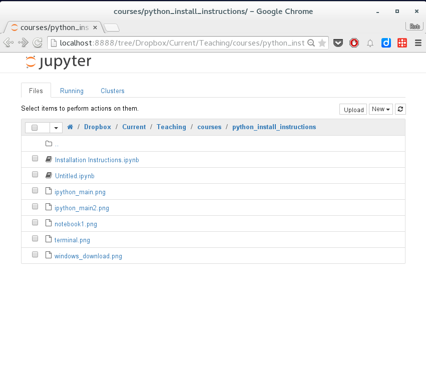
"If you have made it this far, your web browser should pop up and you should see a window like this (note: the actual filenames and folders you will see will reflect the actual information you have on your computer):\n",
"\n",
"\n",
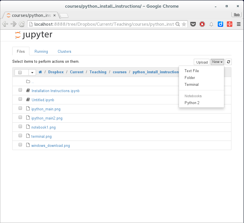
"This listing allows you to see existing and running Ipython Notebooks. You won't have any, so let's create one. You can navigate to a folder of your choosing and create a new notebook by clicking on `New` and then `Python 3` as shown below [Note, the screenshot below is from an old python version and shows `Python 2`):\n",
"\n",
""
]
},
{
"cell_type": "markdown",
"metadata": {},
"source": [
"## Testing the installation\n",
"\n",
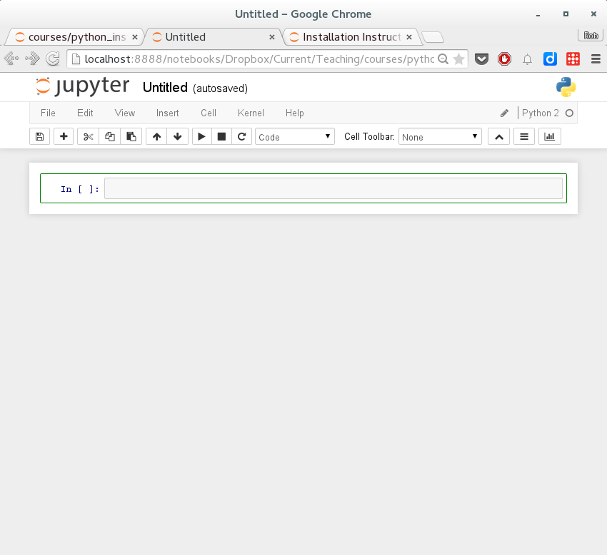
"Having created a new notebook, you should see a window that looks like this:\n",
"\n",
"\n",
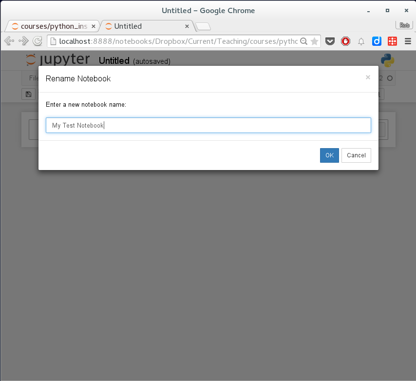
"You can re-name your new untitled notebook by clicking on ``Untitled`` and changing the name:\n",
""
]
},
{
"cell_type": "markdown",
"metadata": {},
"source": [
"Ipython Notebooks have execution blocks where you can enter and execute python code. These blocks look like this:\n",
"\n",
"\n",
"Copy and paste the following code into the first (and only at this point) execution block:\n",
"```\n",
"%matplotlib inline\n",
"import pandas as pd\n",
"import numpy as np\n",
"import matplotlib.pyplot as plt\n",
"import statsmodels.formula.api as sm\n",
"import sympy as sympy\n",
"```\n",
"\n",
"You should see output like this after pressing the `shift enter` keys at the same time to execute the code:"
]
},
{
"cell_type": "code",
"execution_count": 1,
"metadata": {},
"outputs": [],
"source": [
"%matplotlib inline\n",
"import pandas as pd\n",
"import numpy as np\n",
"import matplotlib.pyplot as plt\n",
"import statsmodels.formula.api as sm\n",
"import sympy as sympy"
]
},
{
"cell_type": "markdown",
"metadata": {},
"source": [
"Next, we will make sure things are working. Paste this code into the next execution cell and press ``shift enter``:"
]
},
{
"cell_type": "code",
"execution_count": 2,
"metadata": {},
"outputs": [
{
"data": {
"text/html": [
"
\n",
"\n",
"
\n",
" \n",
"
\n",
"
\n",
"
time
\n",
"
price
\n",
"
\n",
" \n",
" \n",
"
\n",
"
count
\n",
"
100.000000
\n",
"
100.000000
\n",
"
\n",
"
\n",
"
mean
\n",
"
50.500000
\n",
"
9.589623
\n",
"
\n",
"
\n",
"
std
\n",
"
29.011492
\n",
"
3.293449
\n",
"
\n",
"
\n",
"
min
\n",
"
1.000000
\n",
"
3.864494
\n",
"
\n",
"
\n",
"
25%
\n",
"
25.750000
\n",
"
7.160937
\n",
"
\n",
"
\n",
"
50%
\n",
"
50.500000
\n",
"
9.162188
\n",
"
\n",
"
\n",
"
75%
\n",
"
75.250000
\n",
"
11.723528
\n",
"
\n",
"
\n",
"
max
\n",
"
100.000000
\n",
"
19.286071
\n",
"
\n",
" \n",
"
\n",
"
"
],
"text/plain": [
" time price\n",
"count 100.000000 100.000000\n",
"mean 50.500000 9.589623\n",
"std 29.011492 3.293449\n",
"min 1.000000 3.864494\n",
"25% 25.750000 7.160937\n",
"50% 50.500000 9.162188\n",
"75% 75.250000 11.723528\n",
"max 100.000000 19.286071"
]
},
"execution_count": 2,
"metadata": {},
"output_type": "execute_result"
}
],
"source": [
"# create some toy data\n",
"time=np.arange(1,101)\n",
"price = np.random.normal(10,3,(np.size(time)))\n",
"\n",
"# load into pandas dataframe\n",
"df = pd.DataFrame(np.c_[time,price],columns=['time','price'])\n",
"\n",
"# run summary statistics\n",
"df.describe()"
]
},
{
"cell_type": "markdown",
"metadata": {},
"source": [
"We can also visualize our data easily using the pandas package:"
]
},
{
"cell_type": "code",
"execution_count": 5,
"metadata": {},
"outputs": [
{
"data": {
"text/plain": [
""
]
},
"execution_count": 5,
"metadata": {},
"output_type": "execute_result"
},
{
"data": {
"image/png": "iVBORw0KGgoAAAANSUhEUgAAAYQAAAD8CAYAAAB3u9PLAAAABHNCSVQICAgIfAhkiAAAAAlwSFlzAAALEgAACxIB0t1+/AAAADl0RVh0U29mdHdhcmUAbWF0cGxvdGxpYiB2ZXJzaW9uIDIuMi4yLCBodHRwOi8vbWF0cGxvdGxpYi5vcmcvhp/UCwAAD6dJREFUeJzt3X2wHXV9x/H3R6KF4BM0F0yBeNXBB8ooYGRstRVBO1QUsB2tju0wao3jaBVrW+PD+DCddlKf0E47KgpNRKUFFaVCVaSOTP8QDRQhGCyOphBCSaxa8KEi+O0f55d6Eu5N9sa7Z0+S92vmzNnds+fsh8vdfO7unt1NVSFJ0v2GDiBJmg4WgiQJsBAkSY2FIEkCLARJUmMhSJIAC0GS1FgIkiTAQpAkNUuGDtDFsmXLanZ2dugYkrRXueaaa75bVTNd598rCmF2dpb169cPHUOS9ipJ/nMh87vLSJIEWAiSpMZCkCQBFoIkqbEQJEmAhSBJaiwESRJgIUiSGgtBkgTsJWcqa2FmV182yHI3rTltkOVKWhxuIUiSAAtBktRYCJIkwEKQJDUWgiQJsBAkSY2FIEkCLARJUmMhSJIAC0GS1FgIkiTAQpAkNRaCJAmwECRJTW+FkOSoJF9KsjHJjUle06YfmuSKJDe350P6yiBJ6q7PLYR7gNdV1eOAJwOvTHIMsBq4sqqOBq5s45KkgfVWCFV1e1Vd24bvAjYCRwBnAOvabOuAM/vKIEnqbiLHEJLMAscDVwOHV9XtMCoN4LBJZJAk7VrvhZDkgcAngbOr6s4FvG9VkvVJ1m/btq2/gJIkoOdCSHJ/RmXwsar6VJt8R5Ll7fXlwNa53ltV51bVyqpaOTMz02dMSRL9fssowHnAxqp6z9hLlwJnteGzgM/0lUGS1N2SHj/7KcAfATckua5NeyOwBrgoyUuBW4Dn9ZhBktRRb4VQVf8GZJ6XT+lruZKkPeOZypIkwEKQJDUWgiQJsBAkSY2FIEkCLARJUmMhSJIAC0GS1FgIkiTAQpAkNRaCJAmwECRJjYUgSQIsBElSYyFIkgALQZLUWAiSJMBCkCQ1FoIkCbAQJEmNhSBJAiwESVJjIUiSAAtBktRYCJIkwEKQJDUWgiQJsBAkSY2FIEkCLARJUmMhSJIAC0GS1FgIkiTAQpAkNRaCJAmwECRJjYUgSQIsBElS01shJDk/ydYkG8amvS3JbUmua49n9bV8SdLC9LmFsBY4dY7p51TVce1xeY/LlyQtQG+FUFVXAd/r6/MlSYtriGMIr0pyfduldMgAy5ckzWHJhJf3fuAvgWrP7wZeMteMSVYBqwBWrFgxqXz6JcyuvmzoCBO3ac1pQ0eQFs1EtxCq6o6qureqfg58CDhxF/OeW1Urq2rlzMzM5EJK0n5qooWQZPnY6HOBDfPNK0marN52GSW5EDgJWJZkM/BW4KQkxzHaZbQJeHlfy5ckLUxvhVBVL5xj8nl9LU+S9MvxTGVJEmAhSJIaC0GSBHQshCTH9h1EkjSsrgeVP5DkAYyuT/TxqvpBf5GkvceQJ+N5UpwWW6cthKp6KvAi4ChgfZKPJ3lmr8kkSRPV+RhCVd0MvBl4PfA04G+T3JTk9/oKJ0manK7HEB6f5BxgI3Ay8JyqelwbPqfHfJKkCel6DOHvGF176I1V9ZPtE6tqS5I395JMkjRRXQvhWcBPqupegCT3Aw6sqh9X1QW9pZMkTUzXYwhfBA4aG1/apkmS9hFdC+HAqvrh9pE2vLSfSJKkIXQthB8lOWH7SJInAj/ZxfySpL1M12MIZwMXJ9nSxpcDf9BPJEnSEDoVQlV9LcljgccAAW6qqp/1mkySNFELuR/Ck4DZ9p7jk1BVH+kllSRp4joVQpILgEcB1wH3tskFWAiStI/ouoWwEjimqqrPMJKk4XT9ltEG4GF9BpEkDavrFsIy4BtJvgr8dPvEqjq9l1SSpInrWghv6zOEJGl4Xb92+uUkDweOrqovJlkKHNBvNEnSJHW9/PXLgE8AH2yTjgA+3VcoSdLkdd1l9ErgROBqGN0sJ8lhvaXaRwx5e0VJWqiu3zL6aVXdvX0kyRJG5yFIkvYRXQvhy0neCBzU7qV8MfDP/cWSJE1a10JYDWwDbgBeDlzO6P7KkqR9RNdvGf2c0S00P9RvHEnSULpey+g7zHHMoKoeueiJJEmDWMi1jLY7EHgecOjix5EkDaXTMYSq+u+xx21V9V7g5J6zSZImqOsuoxPGRu/HaIvhQb0kkiQNousuo3ePDd8DbAKev+hpJEmD6foto6f3HUSSNKyuu4z+dFevV9V7FieOJGkoC/mW0ZOAS9v4c4CrgFv7CCVJmryF3CDnhKq6CyDJ24CLq+qP+womSZqsrpeuWAHcPTZ+NzC76GkkSYPpuoVwAfDVJJcwOmP5ucBHdvWGJOcDzwa2VtWxbdqhwD8xKpNNwPOr6vt7lFyStKi6npj2V8CLge8DPwBeXFV/vZu3rQVO3WnaauDKqjoauLKNS5KmQNddRgBLgTur6n3A5iSP2NXMVXUV8L2dJp8BrGvD64AzF7B8SVKPut5C863A64E3tEn3Bz66B8s7vKpuB2jP3nVNkqZE1y2E5wKnAz8CqKot9HzpiiSrkqxPsn7btm19LkqSRPdCuLuqinYJ7CQH7+Hy7kiyvH3GcmDrfDNW1blVtbKqVs7MzOzh4iRJXXUthIuSfBB4aJKXAV9kz26WcylwVhs+C/jMHnyGJKkHXa9l9K52L+U7gccAb6mqK3b1niQXAicBy5JsBt4KrGFULi8FbmF0XwVJ0hTYbSEkOQD4fFU9A9hlCYyrqhfO89IpXT9DkjQ5u91lVFX3Aj9O8pAJ5JEkDaTrmcr/C9yQ5AraN40AqurVvaSSJE1c10K4rD0kSfuoXRZCkhVVdUtVrdvVfJKkvd/uthA+DZwAkOSTVfX7/UdaXLOr3bCRpC52d1A5Y8OP7DOIJGlYuyuEmmdYkrSP2d0uoyckuZPRlsJBbZg2XlX14F7TSZImZpeFUFUHTCqIJGlYC7kfgiRpH2YhSJIAC0GS1FgIkiTAQpAkNRaCJAmwECRJjYUgSQIsBElSYyFIkgALQZLUWAiSJMBCkCQ1FoIkCbAQJEmNhSBJAiwESVJjIUiSAAtBktRYCJIkwEKQJDUWgiQJsBAkSc2SoQNI2rvMrr5ssGVvWnPaYMveH7iFIEkCLARJUmMhSJIAC0GS1FgIkiRgoG8ZJdkE3AXcC9xTVSuHyCFJ+oUhv3b69Kr67oDLlySNcZeRJAkYrhAK+EKSa5KsGiiDJGnMULuMnlJVW5IcBlyR5Kaqump8hlYUqwBWrFgxREZJ2q8MsoVQVVva81bgEuDEOeY5t6pWVtXKmZmZSUeUpP3OxAshycFJHrR9GPgdYMOkc0iSdjTELqPDgUuSbF/+x6vqcwPkkCSNmXghVNW3gSdMermSpF3za6eSJMBCkCQ1FoIkCbAQJEmNt9CU9lJD3spS+ya3ECRJgIUgSWosBEkSYCFIkhoLQZIEWAiSpMZCkCQBFoIkqbEQJEmAZypL0m4NeVb4pjWnTWxZbiFIkgALQZLUWAiSJMBCkCQ1FoIkCbAQJEmNhSBJAiwESVJjIUiSAAtBktRYCJIkwEKQJDUWgiQJsBAkSY2FIEkCLARJUmMhSJIAC0GS1FgIkiTAQpAkNRaCJAmwECRJjYUgSQIGKoQkpyb5ZpJvJVk9RAZJ0o4mXghJDgD+Hvhd4BjghUmOmXQOSdKOhthCOBH4VlV9u6ruBv4ROGOAHJKkMUMUwhHArWPjm9s0SdKAlgywzMwxre4zU7IKWNVGf5jkm4uw7GXAdxfhc/owzdlguvNNczaY7nzTnA12ype/GTDJfU3kZ/dL/DcvAx6+kDcMUQibgaPGxo8Etuw8U1WdC5y7mAtOsr6qVi7mZy6Wac4G051vmrPBdOeb5mww3fmmORv8f77ZhbxniF1GXwOOTvKIJA8AXgBcOkAOSdKYiW8hVNU9SV4FfB44ADi/qm6cdA5J0o6G2GVEVV0OXD7Aohd1F9Qim+ZsMN35pjkbTHe+ac4G051vmrPBHuRL1X2O50qS9kNeukKSBOxHhZDkgCT/nuSzQ2fZWZKHJvlEkpuSbEzyG0Nn2i7Ja5PcmGRDkguTHDhwnvOTbE2yYWzaoUmuSHJzez5kirK9s/1/vT7JJUkeOkS2+fKNvfZnSSrJsmnKluRP2mVubkzyjiGyzZcvyXFJvpLkuiTrk5w4ULajknyp/dtxY5LXtOkLXi/2m0IAXgNsHDrEPN4HfK6qHgs8gSnJmeQI4NXAyqo6ltGXAF4wbCrWAqfuNG01cGVVHQ1c2caHsJb7ZrsCOLaqHg/8B/CGSYcas5b75iPJUcAzgVsmHWjMWnbKluTpjK5i8Piq+nXgXQPk2m4t9/3ZvQN4e1UdB7yljQ/hHuB1VfU44MnAK9vlgBa8XuwXhZDkSOA04MNDZ9lZkgcDvw2cB1BVd1fVD4ZNtYMlwEFJlgBLmeOckUmqqquA7+00+QxgXRteB5w50VDNXNmq6gtVdU8b/Qqj824GMc/PDuAc4C+Y4wTRSZkn2yuANVX10zbP1okHa+bJV8CD2/BDGGjdqKrbq+raNnwXoz8oj2AP1ov9ohCA9zL6hf/50EHm8EhgG/APbZfWh5McPHQogKq6jdFfZbcAtwP/U1VfGDbVnA6vqtthtHIAhw2cZz4vAf5l6BDjkpwO3FZVXx86yxweDfxWkquTfDnJk4YOtJOzgXcmuZXRejLk1h8ASWaB44Gr2YP1Yp8vhCTPBrZW1TVDZ5nHEuAE4P1VdTzwI4bb5bGDts/xDOARwK8BByf5w2FT7Z2SvInRpv3Hhs6yXZKlwJsY7e6YRkuAQxjtBvlz4KIkc136ZiivAF5bVUcBr6Vt5Q8lyQOBTwJnV9Wde/IZ+3whAE8BTk+yidGVVU9O8tFhI+1gM7C5qq5u459gVBDT4BnAd6pqW1X9DPgU8JsDZ5rLHUmWA7TnwXYtzCXJWcCzgRfVdH3P+1GMyv7rbf04Erg2ycMGTfULm4FP1chXGW3hD3LQex5nMVonAC5mdCXnQSS5P6My+FhVbc+04PViny+EqnpDVR3ZrunxAuBfq2pq/sqtqv8Cbk3ymDbpFOAbA0Yadwvw5CRL219mpzAlB7x3cimjlZP2/JkBs+wgyanA64HTq+rHQ+cZV1U3VNVhVTXb1o/NwAntd3IafBo4GSDJo4EHMF0X4tsCPK0NnwzcPESItm6eB2ysqveMvbTw9aKq9psHcBLw2aFzzJHrOGA9cD2jleCQoTONZXs7cBOwAbgA+JWB81zI6HjGzxj9A/ZS4FcZfYvi5vZ86BRl+xajy71f1x4fmKaf3U6vbwKWTUs2RgXw0fa7dy1w8jT97ICnAtcAX2e0z/6JA2V7KqMD3NeP/Z49a0/WC89UliQB+8EuI0lSNxaCJAmwECRJjYUgSQIsBElSYyFIkgALQZLUWAiSJAD+D0vzwfnvAnbiAAAAAElFTkSuQmCC\n",
"text/plain": [
""
]
},
"metadata": {},
"output_type": "display_data"
}
],
"source": [
"# plot histogram of price\n",
"df.price.plot(kind='hist')"
]
},
{
"cell_type": "code",
"execution_count": 6,
"metadata": {},
"outputs": [
{
"data": {
"text/plain": [
""
]
},
"execution_count": 6,
"metadata": {},
"output_type": "execute_result"
},
{
"data": {
"image/png": "iVBORw0KGgoAAAANSUhEUgAAAXQAAAD8CAYAAABn919SAAAABHNCSVQICAgIfAhkiAAAAAlwSFlzAAALEgAACxIB0t1+/AAAADl0RVh0U29mdHdhcmUAbWF0cGxvdGxpYiB2ZXJzaW9uIDIuMi4yLCBodHRwOi8vbWF0cGxvdGxpYi5vcmcvhp/UCwAAIABJREFUeJzsvWm4LFlZJvqumHLYO/e8z1x1Tg3UQBVFAYepQEVABEVBvd2KLXIVGluvXLVtp6utj92tctVHr639KNjSOCA02lzwKgiIMlRRUHWqqOnUeGo6857PHnKKad0fEV/EisgVkZHT3pm5432eemqf3LEzIzNXfPGu93u/72Occ+TIkSNHjtGHstcnkCNHjhw5+oM8oOfIkSPHmCAP6Dly5MgxJsgDeo4cOXKMCfKAniNHjhxjgjyg58iRI8eYoG1AZ4xdxRj7F8bYY4yx04yxn/Ifn2OMfZ4x9pT//9nBn26OHDly5EgCa+dDZ4wdBnCYc34/Y6wC4D4AbwfwvwNY55y/nzH2iwBmOee/MOgTzpEjR44ccrRl6JzzS5zz+/2ftwE8BuAogLcB+HP/sD+HF+Rz5MiRI8ceoS1DjxzM2AkAXwZwK4CznPMZ4XcbnPNU2WVhYYGfOHGiqxPNkSNHjv2K++67b5VzvtjuOC3rEzLGJgH8LwA/zTnfYoxl/bv3AngvAFx99dU4depU1pfMkSNHjhwAGGPPZzkuk8uFMabDC+Yf4Zx/wn94ydfXSWdflv0t5/yDnPOTnPOTi4ttbzA5cuTIkaNLZHG5MAB/BuAxzvnvCb/6OwDv8n9+F4BP9f/0cuTIkSNHVmSRXF4D4J0AHmaMPeA/9n8BeD+AjzPG3g3gLIB/NZhTzJEjR44cWdA2oHPO7wSQJJi/ob+nkyNHjhw5ukVeKZojR44cY4I8oOfIkSPHmCAP6Dly5MgxJsgDeo4cOQaK+89u4JELm3t9GvsCeUDPkSPHQPGf//5R/M5nn9jr09gXyFwpmiNHjhzdoG460JWcO+4G8k85R44cA4XpuGjazl6fxr5AztBz5MgxUJi2i6bq7vVp7AvkDD1HjhwDheW4MO08oO8GcoaeI0eOgcK0XWhKHtB3A3lAz5Ejx0Bh2i5UJdfQdwN5QM+RI8dAYTkcipUz9N1AHtBz5MgxMHDOYTp5MN8t5EnRHDlyDAwUzE3HhetmH3eZozvkAT1HjiGC43L80H//Or56ZnWvT6UvsJwwiOdMffDIA3qOHEOE7YaFO8+s4hvnruz1qfQFol2xmVsXB448oOfIMUSoW54bZFyCXzSg506XQSPLTNEPMcaWGWOPCI/dzhj7GmPsAcbYKcbYKwZ7mjly7A80fDeINSbyhPg+mrnTZeDIwtA/DODNscd+G8Cvc85vB/Cr/r9z5MjRIxo+Qx+XyspmLrnsKtoGdM75lwGsxx8GMOX/PA3gYp/PK0eOfYn6mAX0XHLx8iJ3P72GKzVz4K/VrYb+0wB+hzF2DsDvAvil/p1Sjhz7F+PG0COSy5i8p07x5NIO3vGnX8MDu5Do7jag/ziAn+GcXwXgZwD8WdKBjLH3+jr7qZWVlS5fLkeO/QHSmcfF4mfmGnpwUzPUwXtQun2FdwH4hP/z3wBITIpyzj/IOT/JOT+5uLjY5cvlyLE/kEsu4wfb9+Lr2vAG9IsAvsX/+fUAnurP6eTIsb/RGDfbYi65BAxdU9jAX6ttLxfG2EcBvA7AAmPsPIBfA/BvAfwBY0wD0ADw3kGeZI4c+wXjZlsUGfq47Do6Bd3U9F2QXNoGdM75OxJ+9bI+n0uOHPse45YUzStFQ8nFGGLJJUeOHANAoKGPCUOPulz2p4a+m5JLHtBz5BgiNMeZoe9Tl8tuSi55QM+RY4jQ8APg2AT0PCmaSy45cuxX1M3xklxy22IuueTIsW8xdknRnKEHAX2Yfeg5cuQYAEhyGZfgRzemkq7uWw2dhnwMc6Vojhw5BgCSXMbFh245LlSFoWyoMJ1cchk08oCeI8cQgXTmsZFcbBeGqqCgKfuYobtgDFDzgJ4jx/5CY8x86KbtwtAUFHR1bGSkTmE5HLqqgLE8oOfIsa9AhUWOy+G4vM3Rww/TD2YFTdnXLhd9F9g5kAf0HDmGCg1BlhgH2cW0XRQ0BYam7GOG7u6KwwXIA3qOHEMFklyA8QjoluNLLvtaQ+e7UiUK5AE9R46hghjQm2PgCjFtF7rKUNDUXHLZBeQBPUeOIULDclEpeE1Qx4GhmyJDH4P30w1yySVHjn2KhuVgqqQDCAtSRhmW49sW9f0b0O1ccsmRY//BclzYLkelOD4MvWm7vstFHYv30w1Mx92VoiIgD+g5cgwNSD+f9hn6OATAwIe+z22Lu9FpEcgQ0BljH2KMLTPGHok9/j7G2BOMsdOMsd8e3CnmyLE/QJZFklzGoVTecjzb4n7W0IdNcvkwgDeLDzDGvhXA2wDcxjm/BcDv9v/UcuTYXyCGPlX0Avo4BECTJJd93JxrqCQXzvmXAazHHv5xAO/nnDf9Y5YHcG45cuwrjKXk4ssNhupJLpyPfqK3UwyV5JKAGwB8E2Ps64yxLzHGXp50IGPsvYyxU4yxUysrK12+XP9hOS7e9t/uwl1nVvf6VHLkACBKLuOTFLWE5lwuB+wxaGfQKYZNcpFBAzAL4FUAfg7Ax1lC5xnO+Qc55yc55ycXFxe7fLn+Y6Nq4sFzV/DIhc29PpUcOQAADT9pWCmOj23R9D3YBd0LNeMgI3UKa5gklwScB/AJ7uEeAC6Ahf6d1uCx07QB7M8FlqP/eOj8FfzGPzzak6RAvdCnyLY4BknRZsDQVe/f1ui/p05hjkBh0ScBvB4AGGM3ADAAjJR2UfMvnv1qpcrRX3z+0SX86Vee7ant7Thq6KLLBRiftsCdwHb4rkwrArLZFj8K4G4ANzLGzjPG3g3gQwCu9a2MHwPwLj5i2Q5i6ONw0eTYe1AwbvTg5KDxc1NjFNBDl4svuexDp8tuSi5auwM45+9I+NUP9flcdhU1M5dccvQPFMgblhMw7I6fwxwv26LtuHA5/MIiX3IZ8ffUDfJeLruAnaYvuexDxpCj/yDpjnTwbkBJ0ekyFRaN9toMhiMLkst+lDitYZJcxhU1klxG/KLJMRwIGHoPAYtkm3Hp5ULnr6tK4MPerwx92F0uI4/Q5bL/GEOO/oOCcS8MvW56wa6sq9AUNvIBnfq5RySXfbgjziWXXUDgchmjBfZ7n38SP/GR+3Jv/R6AmGdvSVEHusqg+YzWGvHdI0kuBXX/Si6c83xiUTc4fXET3/WHd6LqM+92qI6h5PK505fx6Ycv461/eCfe8+f34umVnb0+pX2D0OXSm+RS9Jmsriojz9ADyUVj+7awiCpj84lFHeKh85t4+MImLm02Mh1fJZfLGDH0huXg9TcdwM9+2w342jPr+I+ffKT9H+XoCxp26HLp+jksB0XDC+iGpow82aCAbqiq4HLZXwyddlm7Jbm0tS2OCohx2262i6DaHL/CoqbtYn7CwPve8AI8dGET59Zre31K+wZUAVnvKaC7KPpM1mtmNdoBnYKZ6HIZ9V1HpyDZKZdcOgRp4padrb6pOoal/w3LQVH3mFBJV3tiizk6A62j3gJ6KLkUtNGXXJqBy4UJGvpov6dOETB0NZdcOgJJKFm3qcHxY7TARIZX1JWegkuOztCPStG65aAkSi4jvjYDyUXz+qED4yVxZkEY0HOG3hFqvoSS1RkQSi7jscA452jaTqBVegx9PN7bKCBLUvTceg1v/L0vYWlLnucRGfo4aOh0LRb8fujAeEmcWWDnkkt3IMZtZ2w5Om6l/5bD4XKEDN1Qc4a+i2hmSIqeWd4J/pOhYbmBG8QYJ5eLqkBXGRgbn+stK8xccukO3TP08Qh69D6IoRf9KevuPhwosNvgnGcqLKLvKMla27AclPSQoY+6D90UkqKMsX05VzSXXLpEtxr6uCwwkleIoZMW20speo5soN0RkJ4UpbVWSwj6YlJ7HHzo8WBW0NR91w89l1y6ROByyczQw6ToiHX+laKVoXtfbS+l6DmyQdzlpeUtKCFIZCKOiG1xDNhsM/ChU0Af/ffUKYhgarnk0hkCH3oGDd20XVgOx4TPYkc9+QSEgaTQwtBH/70NO8QgnqahU+AnebDleeyo5DLq65J2GGRZLOijv+voFFbspjZojE1AJ4ae5SKg4D87YQAYD9mFAglt2en/OUMfPMQgnh7Q0xl63Qwll8K4Si4j/p46RVD6PywBnTH2IcbYsj+dKP67/8AY44yxPZ8nSq6VLJILXVBzfkAf9QsHCIMFsSEKDHlx0eAhBqluNXTPduoGfu1x86EDJLnsr/U4jJLLhwG8Of4gY+wqAN8G4Gyfz6krhJWiWRi6d+xseXwYejPG0Et5QN81ZGbo/u9qEoZOa3AcJZdoQB/t99Qphk5y4Zx/GcC65Fe/D+DnAex5RtF1eRDQ7Qw2vThDH4fMexJDz73ogwexTkNTUE9LihJDl2joJI0Vx8iHTrtlGu5gaMq+qxQdOslFBsbYdwO4wDl/sM/n0xXEoNWJhj43xhp6yNBH/70NOyhIzZb1rjV0spcWR9iHfm69FgyOAYCm4wYedIA09P1FMKwhlFwiYIyVAfwygF/NePx7GWOnGGOnVlZWOn25TBAvkCzNuUhyGWcNvWT4tsWcoQ8cFIxnSkY2l4tEQ6cbb0nwoVsOH6nCsH/9gbvxR/98Jvi3absoCMx0P0ou5rBJLhJcB+AaAA8yxp4DcAzA/YyxQ7KDOecf5Jyf5JyfXFxc7P5MUyBuYTMlRcnlMkYaepyhkx8919AHDwrG02U9PSlKPnRJpWiL5ELtZkeEpXPOsbTViPSpiY9eK+i5y2XQ6LgfOuf8YQAH6N9+UD/JOV/t43l1hAhDz9APvRZo6N509XHYBtKFEkguRh7QdwvNgKFnk1ykDJ0Kw/SwfS7gBXT6TocZDcuFy4GtuhU8ZtpuhJkWNGUs8lWdYOgkF8bYRwHcDeBGxth5xti7B39anUG8QLJILjsxl8s4SC4USHLb4u6jEWjoBhpWcuVx0MtFpqHTDkvotgiMztok7Xy7Eb4303aD9wH4Pd5HZMfRL4gNynYDbRk65/wdbX5/om9n0yXELWwWyaVm2lAYMFUihj76iyyoFKWAHpT+j/57G3ZQMJ4ph+tJxqqDIRhSDd17LOiHro5WQKdd71YjZOjecOSQmXq9XEbj/fQLJLkMs4Y+dIgw9AwBfadpY6KgBRfdbksuZ5a38abf/xI2qmbfnrNpO9AUb2I8AGh+y9I8KTp4UKCe9gN6UnVuqKEnJ0VbNPQRCejE0EXJpWm7MLTwxlbQ919SlHzoQyO5jAKiDL295FJrOpgwtD27aE5f3MKTSzs428eZn15jpygrLOZj6HYFAUMveRJe0k2UiEPdcuDE3CtJksuoWBfpJrUlSi5OVHIxVE9yGSXnTq+Ie/EHjbEI6MTQp4paNoZu2pgoqHs255DOt5/B1ptWFP0687miu4OG5UJXGSYK6XmLtBYB9QTJZVQYLZGqnaYd3Kws24UhSi76aDl3+gHL5TDU0Is/aIxFQKck00zZyKah+5JLENB3WdejLXm3nRDPrddarG85Q987NG1vdBxZRZMYurgTrEm+PyBk6PqI2RbFgqKdRjibIJoU3X9zRS3b3TW5BRiTgF5rOlAYMFnIxtCrccllly8auuC7Dbbf+8dfxQe+9HTksabtBAyIUNLzMXS7AW90nCpYReXrqWm7QZKwGtPZA5eS/x0W+pAUPfXcOv7ya893/fedQCQYlBiV2RaB8bAJZ4XluLvmcAHGJKBXTRsThgZdUzJp6FVfcgm2tbsc9MgR0E1A55xjdaeJlZ1m5PGG5QYMiFDU03uL5OgPmpYnd7VriNa0ncAqG99hNS0HjIVBrx/5nY+fOoff+vRjuzLARbxBUUCPB7O9kjj3EpbL84DeKWpNB+WCCkNlmStFJwrans05JA29m62n53NudUo0bSdwSBByyWV34NkUleDzT3O5ULsJmYZe1NRAa+1HQDdtFzXTwXbCDNN+IsLQ6+E0MCNWKQrss4Au7Mp2A2MR0AOGrmZraFQ1HZQNz4K/F6O+KMh2M++T2H28BWvTcluTokYe0HcDNAs0YOgJ32vTdhMZujh+DuhP6T+t68ubjTZH9g6Z5NKUFBZ5j++fNZlLLl2gZnoMXVMVmFkkl6aNyULY82SUXC70t3GG3rCd1qSolgf03UDDdxilTYlyXQ7TcTHrt5uIl/83rHD8HNCfwiJzFwP6ToShh5KLXEPfRwzd5TlD7xQ100bZ0GCoDHYbRkO904mh78UUlTCgd76w6W+zMvQ8KdqKLzy2hOXt/gW5pu8wCtotSAIWMe0khl63ojfkdgz9zqdW8fD5zdTzor+9vLU7DH2q6F1T27nLJYAnueQMvSPUTAcThppJcqn5AW6yEAb0OAty3MG2La33xNC9i6XFJSFj6LqS90OPoWbaeM9fnML/vOdc356TPvvA5SJh6BTESENvZejh+DmgvYb+n/7+NP7gC0+lntduSi47TQeHposAkl0uRi65DBxjEdCrTRvlghb0kE4D+X/LhbAiL74F/K4/vBP/zz89OZiThWhb7DzY0s0g7mNuWm7gYSYUdVUaXMYZTy5tp7o6lrea4DwqEfQK0r+pf47sRh10ZCSGHt9h2Q5KoobeRnKpNp1I3xQZgoC+Cwy9ZtqYKuqYLGhBUrSlfe4+lFzsXHLpHDXTQVlXoamsreZIF3LA0CU9mp9Z3cEXHl8ezMlCkFy6Sor6Ad1qZej73Yf+yW9cwJt+/8v4ylPJnZyXtz27p6yFbbfwqnTV1P45tMamihoU1jqGrm52Jrk0bSfS2VCG3dTQiVRNFTVsNSy4Lofl8AhDp6Tvfgropu0G/ZV2A2MR0MmGaKgK7Db90OlCDjR0VYEpBFbbcdGwXDx2aauvLE5EvQcfOgXyeEBoWDLJRYXt8pHpB9ILaqaN93/mcQDAF59Inoy1MoCALjpUipr8JkoMvairmDC0FoYel8zaMfS66UQaYclA63q3kqKTBRVTJR3bDSu4Eck19P1DMuKJ4UFj5AM655TkVDNJLhSkqe9GvAMcBUyXAw+euzKQc+7Fh043A9Nxg4udc46mLUmK7qOe6B/40jO4vNXA0ZkS7jyTHNApGVq3+im5OEGwKhqqVEoT2xuXC2qLE6ZhuRGXi6YqUJg8oHPO0bBdbLeRXHY3KepVX08VdWzV7YBE7HeXSy65dAjTcWG7HBOkobdZLJRUnBBdLsIFKLoPTj23MYAz7q30X2SWFBRMxys2kiVFvdfp7QJai1WlDhsuXqnjA19+Gm+97TB++NXH8eTSDpYTghhJLknFP92gabuB3OUlopMll0LA0Fsll7hkZiQMhLAcDsfl2GnaqfkCWtfrVXPgN3XaJVd8ySWYpSlh6KPSErgfyCWXDkHSg8fQWdtCDJpWNCEkRcW/EQP6fWcHFND7oKEDYWItPiCa0I+pRZ87fRkv+y//hDPLO10/x6Dx2//4ODgHfvEtN+E11y8AAO56Wq6jL2/1V3JxXQ7TDhPSSR0uSXIpaApKhtqa1Ja4lAy11YEFhITA5a1uJxGm46LsO2/ofQ8CnHNUTRuTBQ1TJd0L6DLJZR9q6EMnuTDGPsQYW2aMPSI89juMsccZYw8xxv5fxtjMYE8zGVWBceuqEkwISUItkFyIoasRGxUF/MPTRXzj+Y2WvtW9wrTd4By7kVxE/3m8J0xBoqEDyd3/2oFzjj/0p7iT9jxsOH1xE5984CLe+83X4thsGS88PIW5CSMxMRpKLv0J6C2zXBMS0eJNV6qhxyQXADA0VUpQRA06TXYxbRdXz5UBDFZ2oXmiE35SdLthB6MgRcte2BJ4/CVAwjBKLh8G8ObYY58HcCvn/DYATwL4pT6fV2YESc6Cp6E7Lk8NwqShl9tILt9ywyK2mzaeXNpuew5feGwJ/+1fzmQ6X3Gr3zNDb0a1+H5r6HedWcPDF7zilWFt4/rPjy2DMeBHX3MNAEBRGO64bh53nVmVyhH9ToqKzBvwbqoyOSf8jlSUC2rL63uFRdHvT1YjQccS0pwuuxXQQ+eYlxTdqlvB5yIydEVh0FW2vxj6sEkunPMvA1iPPfY5zjmtpK8BODaAc8sECsBet0XvTpjm6qALacKQSy47QkAHgPue92QXzjl+7C9P4Vc/9Qji+JtT5/E/7no20/mKF2MvPnRAlFxCB4UIKnTpVi/+4y+dgepPWhlW3fOe59Zx48EKZv2CHQB47fULWNpq4umVVpmo3xp6ODpOkFwkn1UQ+HWfocfm4Doub6kj0BNsuPUMDN1xOWyXhwF9s97J2+oIVYEkVYoaXA5c8R04cblhv80VNZ3R67b4owA+04fn6QqhDVGFrrQf21Vt2ihoSnDXTGLoNx+ewsJkIQjonz29hM+eXsLXn1lvec5Lm/XMFkeSSVSF9S0pGg5HiGvoflK0i2D80PkruOvMGt5++1EAw7lNth0X9z+/gZefmIs8Tjp6XHYxbRfr/hzXfkkuweg4MSkqY+iC5FI2ogw9PiCaYCQwdJEIUBFPHPR385MFlA0VlzcHJ5ntCDLmVNHrVUOJdEOLyg170WpjL2G70alNg0ZPAZ0x9ssAbAAfSTnmvYyxU4yxUysryXayblEVFhNpVXaKdZGSN4S4hi4+38uOz+C+5zfQsBz8xqcfBQBclDCdS5sNNCw3k95OF/Js2ei6lwttYykhFrK/BA29Czb6J196GpWihh95zQkAw8nQH720harp4BXXRAP6VXNlnJgv464z0YC+6geZSkFr6YXTLcJALTL0tICuYqKgRW/MCTmQJJeL+H0mVYuawg3k0HQRl7cGz9ApKQoAKzvejdNQo+9pL9pV7yWGTnJJAmPsXQDeCuDf8BTvFOf8g5zzk5zzk4uLi92+XCIiDD3DYN2q3zudYGgKXI6gqRclRScLGk4en8PZ9Rre/5nHcW69jm++YRHbDTuyzbUcNxg2EU90yUAX72xZ76rAombaWJwseD83KSmaxNC709CfXa3iM49cxg+/+njQe2QYA/o9z3q7pXhABzyW/rVn1iNrgeSW4wtlL5HXh4R3K0NP0tBDycVj6OFaoVzIRJyhJ7hcxBtGkoYuatiHpooDLS4KjAkFVcLQY5KLpDJ7nGGNguTCGHszgF8A8N2c8/6Nru8C4WLSgg8uLYFXbdqBBx1oLXaoNm0ozLtAX3p8FgDw4a8+hze98CC+76We/HBJuDiWthqg21m8g54MAUOfMFqYXM208e/+8j6c30j+SGumg/lJ6geSztC7TYre//wGOAe+5yVHh7oY5J5n13H1XBkHp4otv3vt9QvYadqR4jBKiB6fmwDQXVI6jjCgq8H/ZZ83rcmCpmCioMFyeEtpfvx9JEouZpaAHtoGD00POKALJKjid1xc8xl63OHhJXqzf+6bdQufeuBCn850d8E5hzVskgtj7KMA7gZwI2PsPGPs3QD+CEAFwOcZYw8wxv5kwOeZiLgPHUBqtag3fi45oO8I04xuPToFQ1NgqAp++TtvxpGZEgCvkIUgXihZAnrdDBk6FYgQnl6u4h9PXw50+6S/X0hi6JJeLkDnejEFusmC3pfJOYMA5xz3PrcuZecAcNLX1R8SWsySZfH4vJco7IfTJbQtep9TKaFSlPI0hhqOqiOWvuQ7UKhbISHJtpglKSreQA5NFbG83ey7BZcgypQkuawmMfQOJZf/78GL+KmPPTC0ttk0OC4H59hVyUVrdwDn/B2Sh/9sAOfSFYihl42Qoaf1RK82nWDRAd5FA4QByxt+EXrU3/3aa3CwUsDx+YnA8SEy9EuRgN4+QFDJOUkZDcsJbjD0XtI075plY7qkw1CVVoYu6bbovUZnwbgp3CD2apB2O5xZ3sFGzcIrTsgD+sKkgbkJI2I7Xd5qgjFPYwf643QJagCo9N8Pwo7Lg/UCIGjNwBgLitqqpoOZcriGDsUZepLkInyfSQxd1NAPTxdhuxxrO00ckOxmeoWYFC1o3uuuBRp6by6XakBaRi+RSsRyNyWXtgF92OF1qVOgKiyz5HJYYELxsVhxBv8Lb74p+PngVBGMAZd6YOjECqmNqhjQibGlMeq66aBkkJc5naHTe+uWoRd1YZD2kDH0e57z9POXJzB0xhhuPFjBE2JA325irmwEskA/nC6NFoYettAV11HTn2oEhDUQtMNa2mqgUtAixwO+PJHC0GfKeiJDFyUXknIubzUGEtDFHIDLvZtVEkM3NCVTrolAa3vY1l8WWH6jwGErLBpq0DxRIGQDaZJLzYxeaPFy5J2m03JhEXRVwYFKAReFIC66XrJYF4kVzlFAFxYqXRhpgYZaBXteZios8gNwjKErij8Eu9OALsgDjDG/Z/xwMaR7n13HYqWAE758IsONhyp48nLYH31lu4HFSiEoh++L5BJn6Akyl9fvxfudyNABjxTE5RYgzbbo/d2BSqEtQzdUFYenPanw0oB09KoZWoENzZOUkgL6iYUyHr24hQ3fPtoORC6Gbf1lAfWVGvqk6DChJrhWNLV9YdFO0464CeJtSsV5ozIcni7h0maUodNzZHK5mCG7AqJbyYBxJwQa1+WoW15nybKhBvIN3RTizZ2A1jF0Dctpq0c2bc8aqfiSQSFh67+XuOfZdbzixBwYS2Y/NxysoGo6uODvqJa3PcmhpEd3RL0g/tknOYvEEYEBQ/df/9KWPKAnFRY1LAcK82S7trZFXcHBaS/nsjSgatGdZtQK7DXo8t5bPJi981Un0LRd/PU9ZzM9N32OI8nQ90ByGfmAXjVtlP0LVA8YelqlaCwp6l+AgeQSc8HEcWSmiEtXohr6NQsT/t+2ZxE1y4GusmDbL1749PdJhUAN2wHnQMnQUC6EDD2u44ooxWx0//ULT+F7//iu1HOMzydNYop7hfMbNVzcbODlJ2ZTj7vx0CQABDr68lYTBwSG3g8NvRlzuSQ5i+gmCYSdPimhv7TZkDp10nzoJV1FpagnM3THty2qChYmCtAUNjCnC3VaJERzVNEQc+OhCl57/QL+4u7nMvVt9MreAAAgAElEQVTpDySXEawupfeXSy4doGaGDF1vI7k0bQeWw+UuF3/BxAuP4jg8XcLFzXqwjb+82cD1B7zAkdXlUtLV4EYiJrhqbZKioue+rIcaetN2oasskoQjFGOl6M+uVnHpSiO97Wp82MKQFYOQC+hkQkKU8IKDFQDAE5d34LocqzteQA9aIvRDQ4/JXWExV/Tz8pKi3u/KgeRiw/brGA7LJBdVTfShF3UVFb8RlgyBq8bfaR0coBe9GpMpaVg00JoUBYB3v/YaLG018emHL7V97qY1wpKLk0suHUNk1IGGnhB8apICjmBwrUOSS7KGDgBHZkpoWC6u1CzYjovl7QauXZwAY1mTojZKhhoEAFHf3mmjodeFgD5RUCMMPa6fE+KFLivbTdguTw3Q4gQeILlJ1F6BAtPxFP0cAKaKOo5MF/Hk0jbWayZsl3sBXe+jhm67YCxkYQFDt+MMPdz1BAzddLC6Y8JxeTJDl/VyMV0Uda+IJ1FyibWv9apFB8fQRZkywtAlwexbbljEtQsT+NCdz6YSC0DU0Idn/WVFLrl0AZpWBLTX0AOLYwpD34ltH+M44jOpi5t1LG834XIvyJd1NQjIaahbLsqGJp2v2M7lIo7PKxtahKHL9HPAc1+I7Caoak25+dCMTMKwSS7rVROGqqTupAg3HKrgicvbQT/wA1PFvkoudDMlLZ++1/hzN63Q5UI7hGrTDoJs3LIIhJJLPOg1/M6MU0UNO01bWvEa75E/yGrRuDOs4leLagoL8jAiFIXhR15zAg+e38T9bWYOBENchmj9ZUUuuXQBcTEFkktCAUXYaTHaywUgOcYb6xYvwRZx2C8uunSlEfqHp4t+f44skouNkq5Kk2cB406UXMhz7zN0M2ToMv0caNXQV7cpoCcHszhDT9Jy9wprVRNzE0ZqQpRw48EKzqzsBL1M+i+5RD+rxKSo4HIRXTaXN+VFRUAYjOMSYsPyrKuVog7O5cn4+MSgQTL0nVjeiSSXuH4u4vtedgxTRQ0fuvO51OfeDdvi8lYjs+umE+SSSxeoNUOG3lZyESQLglgpKla8JYEY+qXNenAxHp4uYrKgZbIt0o6iKNmat2PoFJhLhuox9GbI0OMedEJRGLhQbdrBTWC7mTwYIX6DiDcw22us+wE9C244WIFpu7jXHyd4oFIM5Kn+SC7RzyrVtuivNd2391VNO7FKFBAcWLGbad2ipKi3TmU6esDQ/eZYi5UCaqbTlbPHtF380iceTmT4XlK0VXJJC2RlQ8Mbbj6Ib7Rh6LthW/yxv7oPvyJpi90rcsmlC0QYept+6BQAS5KAbtqu0Kg/OaAvTBagqwwXNxuBffHwVAkTBS1zYVHJUKXzPkXGnfS3gM/QDRU1y/EGRLdh6PR8q8Js0DSGHr9BJFUs7hXWqmbQz6YdbjzkJUbv9FvpLlYKUBTm71z6YFuMMXRaW3FXhlhYBHh5nLrp4NJmA7rKgroEEUltF7xhGGogbch09DhDn/dvgKvbnTPRp1d28NF7zuIrT8m7pbYmRfXIayehUtTa7pJ2w+VyYaOOM0v9H7Fo55JLZ3BcjoYVzk3U2vRDlzN0klzcsOItJaCTY+DSlToubTZQNlRMlTSUDTWTbbHhsytiiREfepMYepscgKGiXNDAubfg40FFhNcsyns+0X+edvOJJ1mHT0NvZmbo1x+YBGPAIxc3USloQcCN9ySP46HzV/DE5fbTqhpW1BGU1D/Hs4KGx5X9wrClrQYOVIpSrVlX5QHd+77TGXo8oFP/n9Vq5z1RiNXL1ow4T5RA59VulmZJT/8OANHlMpj1xznHlZqFs+u1tgnaTkE7q5Fon7tXWN1p4qt+n2taaFkrRWtWa0APXC62I/SkSNbQAeDIdAkXrzSCCj/GGCYLrXMipecQl1w6YOh1ISlKOn/VtFu2/SLEKfRiQE+Th+JJ1mGzLa7vZJdcirqKE/MT4BxYnCpEHk9jh//xk4/gNz/9WNvnF6UU73nl7Rbin+mE37rh8mZDalkEkhl6w3JiAV3C0B0HmhJaWSmgU4+VTkBERTaQum55tREyH3o7hl4yvFa6aW2Mw8KiwUguVdOB6bioWw7W+qyj01yGoRoSPWz4i7ufx7/5s6/j+bVqZJ4o0F5yoS12SUjgiBdNNYPkAgCHZ4q4uFnHxc16cDF2JrloQRCQVYpm8aGXhOKUNIYuDi1e2ckW0OMMfZhsiw3LQdV0AgkhC2446NUJHKiEAb1syPuWE7YbNq7U2l/gDcuJtC2W7byAVsmlbGiomg4ubzVwsF1Ad6LP5dUyKIHkItXQLTcSUEmiWtvpnqHLXmdHknea6oChA+ltjKmGYlDrT0yGnlvvbyfwICmq5ZJLIjaqJjgHPvL1s5F5okAHkotwAarC4NosSVHAKy5a2mrg4pU6Dk2Vgr/JZFv0XS6K4vVIERdztdkmKSqMKsvO0FWfRfEOJJfBMPQzyzuRtgndgEbIzU0U2hwZ4ka/wOhAJQyc7SSXmukE5etpaNhuRHKh71WeFA2P8+oIPIYusywCSGyM1rA92W6q5K1T2XmaTjSg045mtYuAHjB0yZqRDefohKED6cnpQZf+bwg37XMb/Z3qFEguSs7QE0Hby4+fOhdc3CShtOuHXhNcIiIM1ZsrmiUpCnjl/5bDsbTVxJEZn6HHptDIwHnYiwXwJgxF55mmFxbVTBuqwmCoSuClr5l2OkM3VHDuLa7VnVB7Tpdc4i6X/tgWf+pj38Cvfep0T88RBvQOGPohCujhTaDUhqHXTBtb9WQnEKFpOS2Tokp6tEUs594wC5Ghl3QNlzcbqFtOouSSZFv0OoyG04GkkkuLFKSiUtCw2oXkkqahy0gQMfR2ycAg35DwPdD1AgxOctmohZ9dvxl6LrlkwHbD6+x2pWbhf957DkC4mBjz2Hay5OI1NSrELsCCrsJ0nI4YOuGQILnUTCdVD2zaLlwe3lAKggPF8RtvKcy7GGXPQ50WGWMhQ286LaX6IgKt3nSxst3EQb+wZieFfTatKOv0elj3fkFdqVl4PEOiMQ2kc2Z1uQACQxc09FIbDb1uOdhqWG0TZaK/nFDUlUiQCiyEMQ2dmobJqkQBuYbu+lW+RV1FQVOgqywxKRpnyAuVQqpOvLzdwE/+9f0tgZu0cxkJkJGgrC4Xug6SckZeUZX386BcLqLkkjYprBvkkksGbDUs3H7VDF5wYBKf9EdTiUlOXVVSJZcJQ2spSCn4TJkWbrukqMio6Gda0GmJ0XrMZSMmLCm4BIMvJIyk1nQEl0aUocdvUoTAHml7XRYXKwVP7084T9flMB1Jc64+MPS65eDcRq2nCs1136XRCUO/bnESP//mG/FdLz4SPCZW2sZhOS4sh8NyeNvhII0Ehi5+f/FB0vT6BJkHHZAHdHqukuHd2L0GXa0MvWm7LcxwfsJI1dDvfXYDf//QJTx+eSvyOLmvZAE9MCZIk6Lp11G7FgziZz9oyeX4fBnn1vsruVjDKLkwxj7EGFtmjD0iPDbHGPs8Y+wp///pbe/6iO2GjUpRxztffTzYioqLSVNYouRSt+wWuQUINeKdpg1dZYl6NOHoTMjQia0HU4dSdHRy2dBCLmqhpZAumnlfG5YFvZog19BNp2Y6LdY5EeK2dmW7icXJgl8EJT/PcKRatMVwP5JSddNzRDy90r3nl1wanSRFFYXhJ153fWRnlSa5iAEmqVcKoRnT0IHW/jni9CCCqDm309DFpCjd+OkmUilq2KrLC4viAXV+0kjV0ImZxxk/ER2Z5BIOVY9KdIaqtJ2l2a5iV9wVDjIpyhhw65FpnOs7Qx9OyeXDAN4ce+wXAXyBc/4CAF/w/70r2G7YmCpq+J6XHA0uirgNMbGXi1BVKoJcHPE2oEmYKesB8w1dLmGSMgn1mIZfFJgcXTTEPGWLvG7aAbOj/1ebdot1ToRYubiyQwxdTUyKhq14owzd5emj/dpB1EPPLHcf0NerJlSFBdv6blHS1eAGG4cYjNvp6A3Lafns45bIcESg4HIR1lmS5CLzoTes6BryOi7KbIuta2J+spBqW6wGWnn0cyEWLmPoMpnS2zlo7SWXNjNvowx9cBr6dEnH1fNlXLxS7+vc1aGUXDjnXwawHnv4bQD+3P/5zwG8vc/nlYithoWpko5KUcf3vPQoAKBSCC/udpJLSdLrnErb4z0pksAYw5HpEoq6gml/ezkhBNgkiD5yICq50N+RNizTFcVGZHQDoaROXMcl0EVzeasBy+FYrPgMvc20+KiGLndbrO00MxdjiH8rzvnsFOtVE7NlQ1qI0wnSbIuiFJPG0Dnn0t1RPCkaauiCy8X/HucnjMTAZ0g+94Ch+89VKch7ojctp1VDnyxgvWYmBq1qIK1YscedyP9lfxMnQtcsTOCIsCOSIWDoSZKLRLbqNzZqJubKBq6aLcNyeF/73Qyl5JKAg5zzSwDg//9A0oGMsfcyxk4xxk6trMhLh7PCdTl2mnZQUPFz334TPvDOl2G6HA/oyZKLjKGT5CIOiG6HIzMlHJ4uBXo8Leg094jYXAuIVnHSNp8KQGTaLbUNAEK/M7k+2jH0834Gf2HSSO07E/T3jtkWgShTXK+aePVv/TP+6bHlxPcbP3fCUz0w9LWqiYUOEqJJoKIWWXCLSC4SOYNguxwub53lWtSjtsWgN7naytCT9HMg2paCQMGPvtepkrwnuoyhL0wa4Dxq1RMRJj+zM3R6rBy7qf3Ve16JX3jLTS3Hi6DBNIkB3dqdgD5T1nHVnHfz6afTJezlMkQMvVdwzj/IOT/JOT+5uLjY03NVTRuch6XF0yUd337LocgxmsoSE3giwxVBkos3bzRdPyf89BtfgP/41puDfweSSwYNnS7Ggqa2MHQKVnLJJTx/RWEoG2oQ0JNdLt5XTB7bdklRWQIvLHAJP9e1nSZMx83MtsX306vk0klCNAnlFP1WfCyNoSdNiioZaiwY+cfprRp6kn4OhJ+7SFDouWjnlZQUNaVJUb/8P0FHDxh6XEMPKkXtlh1ZtWmjqCst5e1FXW3blKroD9ROkr6I1BQGONN2o2phbsJj6EC/A7o3eCZLV9B+oduAvsQYOwwA/v+z0bQeQUykkqKfGqqSqPXStKA4CkJSNIuGDnjTcl5/08Hg3xOCLzwJDYnLJZhlapLkkpYUtSPuiLKhBWwrMSnqv9bZNW+hHqCA3gFDD/rdRKYrecdl7bFN7+fahQk8v1ZNtKq1Q78CepoHupZRQ6eA08rQ4xp6a1KU1kBSlSggzrsVkqJmVBJLmlpkSnrkLwTVogkMXQjcImhNc97qSKmaTuZdbRxBpWgbhj5d0gdnW6yZmCkbODJTAmP9D+i7KbcA3Qf0vwPwLv/ndwH4VH9OJx1hQE9eQGmSSxJDp6n2nUgucUxmklziAT1kcjRNKS0pKtoWAW9XQBdnouTiB2PK4C9OFlEpJI8uk7FOWQk6nV9WzZGe90XHpuFybxReN1jbaXbkcEkC5VJkAb0e0dDTC7CA1vyF+L16xyXbFrMwdHFnFCRFBYa+Y7YOuZDaFiezMfQkl4t4jPjvrCQojnZJ0boQ0NNss8vbDbzqN7+AU8/FU33tsVHzCIKhKTg8Vexrtajl8F2VW4BstsWPArgbwI2MsfOMsXcDeD+Ab2OMPQXg2/x/Dxy0tUxj6GmFRd78UXlS1PS7LZYzJEVlCG2LKQE95lAo6krQq4JY0UKbpKhod+uIoa/XYKgKpkoaJgoamrYr3cmESdFo+1zxd0B4sWWdJE83sxcdnQbQnY5uOS62GnZHZf9JCIZMWDJvdWcMPX4zLQm5ESC030Vsi75El6ahy3IX9dgOaqrodd3cibFqaWHRJJX/J2no8orQWtMO1sC2LKB3ec1oqmdvTPahZ2PoZ5Z2cHmrgT/9yjMdvX7d9Pogzfg5uGNz5b4z9HZOn36j7TfBOX9Hwq/e0OdzaYssDF1L8UzXTbsleQOEkkvNdCJ+2k5Az5vWzyVoDhbxofsM3V/UST50168kFV06E4aKp1eyJUW3GzaOznhJXNEzP12O/l0jpvOLzx2xz3UqufjPe8uRaSgMONOF04Wq+ub6lBQF5EUt9JjCsmnorT50RSq5iDfJ6xYn8eJj03h5yqBrTWFgLCmgh5IL4N14RCtnvJcL4FVwagpLLC6iQC6rFF2sFHDhSr3ldzs97GqB1nyDCAri0yU9tXZh1V8X//TYctABNQuIDM36veivmi3jzjO9GTdEeBr6aEguewK6uKZSArqhKrAlzgXOeaQwJ/I3gsul2+0jJSlrqbZFb4GGtkVvMXPOUW3a0BQWVNnFFzlZuMTzLxe04GJvlxQFvNJvICwCkU0tkum9Mtui2MExaUckgm5Q0yUdJ+Yn8GQXAwWCsv8+augy/ZbOdbFSSHW5yCye9NyOy4PPRSa5zJQNfOonX4trFiYSn58x1tIzvBnb5SV1XDRjzcAAb43OTxptNfQ4C6+ZdtA2IS4pesMtuiNBQOuIRBG05qdLeqrLhW5QjsuDdiBZ0BLQ50pY2mp2nd+Jw3Z4MOd4tzBSAT1LUjRJcmlYXl+IJB/6dsOC7fKuAzqAVPcI4G3vDU0JelQXda9gx3J4oO+H7ovoe5AN5yhLWHQchqqALNuLkxTQvc9P5siRsc60rT/n0T7rSRALYq4/MImnljtn6N005kpCOQNDPzRVTGXoMikFaB1DJyssyorZshFpIBVn6FMJAb1pt/rQAW8HuJYw5EImuZi21wbhoN+pMr5mqk1bKmNmRclILvCiNTPVNqCbUBjwmuvn8bF7z2YugNuoep/rrC+5kNOFeuz0CjNn6OnImhSVSS5xD7iIgh4mUnvZPqaV1ANR2yEgNM4SErJ00ccTRUGVqS4y9NbnioMxFvxu0WfoxKhkCVwZQ5cGdCEQZkmM1oVk3gsOTuK5tVrH5dz9ZOihhi53ExmqgtkJI11Dt+WSC63PTT8QN61Whp4VsxN6xDceuFyE0n8g2nHRdb0+NLKS8/lJAyuJDL3Vb07XTcjQY0VHpo3JLjV0oA1DFyQXx+WJgdrrIlrAO191HJc2G/jiE9lkE/pciSBcNddf66LltCamB40RC+gWVH8eZBKSKkWTWucC0YKPXhi6N4Yu3eUinju5IxqWEyRsvQCstGz7wvFzooYe/pzUPhcIbwKLvvY8mZLADVwusW6LQFRyEc9vKYOOLn7+NxyswHE5nltLd7qcW6/hs6cvB/9e3+m8MVcSAhYt2VHV/QKuqaKe7nJJsC0e8J0ry9ve5yLrtpgVs2Uj2JkA3k1EV1ng+5aNoSNHiIyhL04WkjV0Sc8WeoxaD8cJS3yeaKdI09Abljd1iW6+SU6X1R2v2OwNNx/EgUoBH/n685lemwL6jCC5AP3ri55LLm3gNeZq7ZYoQleZVEMnhpjE0AndJkWB9lOLKFAQiGVRL3ZysMhYi1RyKbQGXRniDH2ymGyxlLpcUmyLQDaGLtrtrj/gTRB6qo2O/tuffQL/7q/uCyYHrfuNlGYkA5U7RTnFtkjy11RJy8bQY589WRGXtrzASZJLN2xtbsKITE6iXuiEiqQnOgU+mcSTpKFbjhvsmMSbA+WEDgSSS/g716V5or1p6Em1GzQ7tSBcJzKsVZv+8HYFP/Dyq/DFJ1cytcIlyYVcLgcrRRiqElRV94pccmmD7YaVKrcAPkOXSi4pAT0ySaY3ySW1OZeVILlYDmpC4y1Zr+54610gO0On3wWSi5ES0C0HjEWDj1xycTFZ0GCoSjbJxXSC6VDXLXqDm9N09Kbt4F8eXwbnwNee8fzFa34fF7XHPi5AuuQSZejJPdED22Lss6dmW+QAIk94N/1nWhi6Fd3lBS4XIQg3E+yUgOdFr/vrTQQF6pmyHrG0EkNfqBhgLBrQN+sWOO/tBlsy1MSh6HXLQVFXgt1iko6+tmMGPZC+56XHwDnw5SdX2772Rs1EpagFQVdRGI7OlvrWdTF3ubTBdsOONOKSQdcUmJLColpgGWwN2IbWH8nFY+gppf+mHfSvAMILrmG5EbdAUbINDW9IYqVoNoZOu4KAoadJLn7nRnEXFFYsRpOiZUPFgalCJsml7gci0vSvniunMvS7n14Lbjh3P+1dnP2qEgXgv8ckhm77DF1P7YlOSdE4Q58t6zBUBUskuaT0q2+H2bKBrYYdyIjxZmBFXYWhKpHkbZrkQvmH1e0oS6fAHU9+EkOfMDRMGtGCtG6GjcRR0tNsi06UoSeU/3vFZt7apgli6wmJXxEbNTNwuBCuW5zAY5d6G8JCsIexsGiYQJJLGnRF7nKhC1dmsRIvtl6SohOGmlopWjcdFBOSonGG3hrQ/RuSId9NpAUMCjiLk+F0JUAe0JtW63xSYqAR26Lp9ZY/PF3MxNBrMbnp5kNTeOjClcTjP3t6CROGildeM4e7n1kD4AWQfgV0sgQmSi66FjhINhNkl0aCbZExFrnRNW2nK/0cAOYmvHO44idY61Zr+4p4+T/deGUBnayrq7GAR2uBkp9kaQ2HvmgtkmI/XEepkotNAT2ZoddNb2j4QsU7h4KmYrKgYb3afnzgRs3CbOzcX3XtPJ5drfY8+xbIGXpbbDWsVMsi4Ekusmx4NVVy6R9DT/Oh0wg5gii5VIXGYPFeIIBccqGf223nKZDSojc0BYamtPiNvXNpnU+aVCla0lUcnCpmKi6KSwUnT8zi3Hody5KbgeNyfP7RJbzupgP41psO4MmlHaxsN7FeNfvicCGUEyxzXgGXOIQ5IaAn2BYBT0cPNfRWT3hWUMChBF7DciOkAPBsfbKALnvNBZ/JxnV0CtQkFwUMXXCHTRTUiKTYzfSoONIGjdBaTNPQqY3BglA9HHcGJWGjagaWRcKrr5sH4O0Qe4Xp8Dygp4GGW6RB1+S9XIIqTakPXWDoPViwPB968lzRVg09lFxqzZiGniUp6h/fjv0RaxHlmsmEBG7DbmXocsnFS1gdmvIYeru+6PHGaCf9CslTz2+0HPuNsxtY3Wni2285hDvoAntmra+SC5AcTIKkqE8ekhKjadr4wali0BYhbQBJO8z5kgCx4bpk5F18yEVaEnY+KP+PM/TQew+E9kR6fKKgYbKoR1wuoY20+1YMnoae7HIpaqo0Kd9yDoLsMxfLOxB+9uMP4nOCa4p6oYu4+dAUZss67jrTe0C3/W6Lu4kRC+jZkqLecNlogAkCorT0P9rwqltMpCTaAInLRShAqVmh/ctj6PHCIonkQsOm27C/g1MFnFgoR8+1oEr1/qaEoSsKg6EqUduiH6APTRfRsNzUikp6jyKzvOXIFIq6gnslDZU+e/oydJXhdTcu4pYj06gUNdz51Ao2an1m6Lp8rmiQFPWrdmUM3XU5HrmwmbheIgFdMmwiKyjheCVg6E6L9bYTyWU+6LgYC+gmMfSoPVFk6JMFFTvCZ0GtGGYnup8eVdJVf36rrBjQaetyofdBjce884k6gwDvJve/7j8fqSTdqJotCV1FYXj1dfO4++nVzMNbkpBLLingnIZbtJFcfLYUty6m+dBpwRS01r7OnaBdg664D5207c2aCc7DAC3z5tZMz5MrG5KQ5nABgF/6jpvx4R95RfRcDXnHRdIt4zA0pSUpWjLU0NHRRkf3GHp4nrqq4ParZnBfjKFzzvHZ00u447oFTBV1qArDq66dx+ceXQLn/fGgE4oJDosgKRr0SWn9nP7vzz6Orzy1ive9/gXS5z44VUDV9KZgNW03caJUO9D7JU2YWKsIb2qRkBRNCegFTUWlqLU06Ao1dJ+hN6Lj6MqGhgkjmvRfq5p+MVz3JIh2nLLEaCC5pLhcZDNm58oG1mMBnRj7qec34Lrc665qOkGOQsSrr1vAxc0Gnl/rze1i5ZJLMqqmA5enV4kCnuQCeBlmEXXTgcLkeict/F4SouLfywI6NdeSSS60baQAXZIUFlFSUXSf0A0gqUpUPK+Fyei2uFKUSy5JjgxDU1p86MTQgQwB3WrtZHny+BxOX9yKsOQnlrZxdr0WGVxyx3XzQVJwbrL3TouEsq5KC4s8yUVLZOgfu+csPvClZ/DOVx3Hj7zmhPS5g89ls+H1VenywiaPNGnCdQlD9/zygm0xxYcOeFOx1qrtNHTv3zXTG2ChKqxl0lU/JLCwwEsS0G0HhTYulxXS0GMMfSOWFCVXz2bdwlPLO8F6klkuSea76+n21sc0WLnkkowsrXMBYbCuE5csvItUVpREDKOXhKj491Ipw2cXooZPzINYRqSwSJIUjSd06QbQjT6b1HcmkaHHWipQgUtQRNMmMSpzZ7zsxCwcl+OBs6Hb5TMPXwZjwBtfGE41vOO6heDnvidFY4HEcTmatouSrkY6GRLufnoNv/LJR/AtNyzi177rhYlFblSIs7zV6MnlUtRVTAiTqeqmK2k1EGXowci7hHUxP2FgdTsuufi2xVgTrqoZtsedLGqxpGjvAT1tclTD9HYjSTNtAe/amTDUyE1utqz7O6PwOUVXz73Prbc05hJx7cIEDk0V8dWExOizq1V8/FT7JmC55JKCLH1cAMDw74hxTa5u2VK5BQiTij0HdCO5R4qslwwxdLpYxS6MLUlRCcPNytCl55owV7SRwNALutJS+l8ylI4kl/h5vvTqWTAWJkYbloOPfP15vPb6hSAgAsANByeDQN53ySX2OYsVxQVNRVFXIkU7H7rrWSxMFvBHP/iSVHlO3Ln0khQFiHF6a6TpF9uIqBS9ZDy5u9IqRQFi6K22RcZCpktro9Z0gorkCX+4OGnLazu95zTShlw0bBclQ5EOyyasVZsR/RwInUFXhKZmdAPTVYZTz60H15xM/2eM4Y7r5vG1p9ekBoc//coz+Pm/fSh1OhmQSy6pIAZC2+Ak0EUWD+hJ04qA0A0wkfD7rEjT0AMNX+xiqHrFLXRxibbFpu1GFlPdtFsYbuBy6SJYTBpay4BpFpcAACAASURBVOxIgDzTGRi6z7gNTcH8hIFLWRi6ET3P6ZKOGw9WgoD+sXvOYnXHbNGlGWOBnay/SdHWnVD8xjtV1CMM/emVHdx+1UzbnSL1PlnaavZkWwS8m1hEcol9P+TGoSAcaOiq/DVl5f/VpoMJw6uaLGhK2BtdZOgFDba/gwH6JLmkdL2kfEGaD12sEiXEnUFAKGvecd0C7n1uIwj2MoYOePbFtaqJJyR9+09f2ASAthq75bij1cuFMfYzjLHTjLFHGGMfZYxl6yzfBbYyMnS6I8Y19LRpRH1j6BTQZc4JqzUpyxhDUVNbGDod0xC2jLIbkqEp0FXWFUOfTNHQ40k3ei0KFJzzSGARHR1JqJvyz/9lx2dx//MbaFgO/uRLz+AV18zhFde0Dn341yevwh3XzbewsV4gk1yCrpb+uU6V9EBDtxwXZ9dquHYxuYc5YaKgoVLQsESSSw8MfaZsYL1mwXJc2C5P7O5Iu1jZUGoR85MFrNdMOAJh8GYBeM87WdCCGgVx3RHhqTY9lr5eNXseNkKus3hfes556HKhwjYJi18VqkQJgXdfCOir202UdBXfcsMiLlyp49GLWwCSd3x3XO/JfHHZxXJcPHbZC/LPtRmjOFLdFhljRwH8nwBOcs5vBaAC+IF+nVgctFjb+tD9O2JcQ69bdiJDJwbQv6RouPBoeyorDAI82YUCOl1QwfAFwYFRTRifVxKSRp0gyTOfpPfSVCfvGK+3PLGrQ9PpxUV0A5DdeF5+Yg47TRu/8Q+P4fJWA+97/fXS5/jmGxbx1//2VX3p40IoGVpbv/9UMUw4nl2vwXY5rl2czPT8B6e9G13Tah3Y3Anmyjo2qmbLPFEC7RboxhMydPlrLk4a4DzKYKtmONxFvNmLQ18mi2Ef/Z2mDdNxe5dcEjR0y+FwOaKFRRKGvrpjYrESY+jkDKpFGfr8pBGQhc896vnRZ8ryndbRmRJOzJfx1TPRxOiZ5Z3g830uhaE7rnf+oya5aABKjDENQBnAxd5PSY6sSVGjG8lFI4bem+RCWiNdDJ/8xgW86re+gEcubCbaJot6yNAnhMIiILrIk8bnTZX0rnYW1CEv7plvZGDowc0pI0MPEsKS83/Z8VkAwF9+7XncftUMXnv9Qssxg0JJV2E60dmq8e9JZOjPrHiMLAtDB7wEY6ihd7+2SEMPhltIXC5AaK9Msy0CoWdb1NHF2aATghwnXjfipKuw7L+3HROtifhOSew1L6tUBjzn2HpVwtDLEoa+43VkvOlQBROGiieXdjBhqKnfyx3XL+CeZ9cj6+MRX25RFZbK0Cn+jIzkwjm/AOB3AZwFcAnAJuf8c/06sTiyJkUDDd1utS0m9VEvaH2SXGJdDD9271ksbTXxrg/dEyyE+DkUdRVEkun1ic2J7DHphvT73387fvJb5aw29Vz914rr6EkM3dDUwA4Xl48OTxexVjUTmyeFwzlan/fYbClwyrzv9dentkbuN2QOi/jNaroUaujP+HMtr1vIyNCniljeavYsucyVDWw37eAaiFeKTsVa6LYN6BNUXCQwdKE53GRRk7pcRBfXerXV/90Nkhi62JefMebvEKPHXKlbcHlrczBi3WI/F+qZrqkKXuqTiHZdIu+4bh7bTRsP+9cuAJy+uIWyoeK2Y9Op/fwpoI+S5DIL4G0ArgFwBMAEY+yHJMe9lzF2ijF2amWl+wGsWYZbAKHkYrnZGbqmMCxMGjg2W5b+Pivo/Gqmjc2ahXuf28B3vfgIGAN+8zOPAUCLjixe6HR+oeQSDTQyl87LT8zhRMpcyiSQPCQ6XRx/0o2UoQtJ0fgYNArIy1vyDne1wDnSesNkjOENNx/Ay47P4vU3HWj5/SARBJPIjTM6SEQccvHMShXzEwamE7bpcdDOpR8uFwC4dKUROW9Cq4buQmHeupaBGLpY/h9Pfia5XACPzYcukf64XOJ1F8HwEP9zixe2AfIqUcCTOaaKWqSfCzF0AMFg7nYVrq++1kvEizr66YubeOHhKVy7MNkS0J9dreLff/wB1E0naD8ySpLLGwE8yzlf4ZxbAD4B4I74QZzzD3LOT3LOTy4uLnb9YlmGWwCC5GK3BnRZHxfACypf+Pevww+/+njX50eY8MfQffHJZTgux4++5gT+8t2vRMW/GFo1dO/fqsKCi17GWtJuSN1AVgQVzhNNsi16v4+Pwzs4TQMd5LILHR+XCgi/8T0vwt/82Kt3lZ0D8rmi8d0HDbngnOOZ1R1cl1E/B7wbne1ycI6uK0WBUEK46HcAjN9wp+IauuPCiLVAFrEwKWPoglYu9PkRAz2t4e2m3bdxgCXJdwC0zrYtaGqL5BIUFUnOQXQGedJM6IY5ecJj6EkOF8K8L9F81S8wcl2O0xe3cOvRaVyzUMbSVjNiXfy7By7iE/dfwBceXwpkmpGRXOBJLa9ijJWZt3LeAOCx/pxWK7K0zgXCStF4g666mZwUBYDpst6Xu6nXI8XG5x9dwsJkAS8+NoObD0/hr97zSrzzVcdxZKYUOZ6CeFmoAg00dH+RU5Vp0g2pu/NsZeiyeaLBeQoMvRELesTQk6yLSck8Ed0Mf+gVslxFa1JUh+1//s+sVDPr50BYpAN0Zy0lEJNMYuiTMYZu2unuiqmiDk1hMYYeSi5ESmzHRcNyg92KjKH3bFvU5JWi9diaKWhKSy8XuiFRS2ARM0KDrit1C47LA4b+kqtmoSmsbUAHPJvjqec8F9aza1XUTAe3HJnC8XlvHYjWxYfOewVyn3n4cmDKGBmGzjn/OoC/BXA/gIf95/pgn86rBdsNq+1wCyDcZopJUc65X5jTP4abhAlDw5W6hS89sYI33nwgCFS3HZvBf377rS0uDWIg0elD0W3oFV/DnWnjwe8EMsklzopERJKisYvtsD9U4NmEJFH8+GGBjB22BHT/Mz+7XsNa1ewwoIcu3p40dD9oXvSn0ce/H11VUNLVQOtv2i6MlGSforAWL7qYFK0UNew0rUAqm0iQXAqa0vM1pSjeDN1WDT3aa17cIRICyaUNQ49LMyVDxS++5SZ8/8uvant+r7l+Hk3bxf1nN4I8mMfQKaB7a55zjgfPe7//58eXgwT1yGjoAMA5/zXO+U2c81s55+/knLcfE9IltrIydInLpWF5NrukStF+YrKg4Z5n17DdtPHGmw+2PZ7kDXE+aFxyIUsgVR/26zyBqOSSNsxYtC0GEooestjbr5oJrGBxhM6R4apjk80Vrce6WpKcQe0Jrs2YEAXiAb2HwqK45CL5fqZKWsSH3u4GMj8RVou6Lg+GlAMeufA6aHo3iIChC5XQVCXaD5lM1i46Lv/JJJe1qgklYcbsbDns5xL2ewmPe883XYvXZHBUveKaOagKw1fPrOH0xS0YmoLrD0zi+LyXb3t21WPoFzcbWN1p4i23HkLdcvBPjy0BGC3JZVfhSS7tGaohkVxI55roo2SRhImCGnSJy7JgsjB00qbFANH7eaZo6O1si5IiqbfedhiPXNiSWrlCzX3wn38nCDV0YSiyP/uUmBVZAh845wf0Dhj6YqUAine9+NApYBFDl+10KkU9mDJkZkjCzk8aQcdFYuKTARP3/r+8Ha1g1vydwE7Dxnq12XNREaFsaIkuF7oWDE1pCeirO16lqqw2YW5CDySXQJrpoiitUtRx27FpfPXpVTxyYRM3HapAVxVUijoWJo2AoT/kr4/3fNO1mJ8w8MkHLgAYIcllt7FVt9oWFQFyhp7WOrffIJbz2usXM71eUYteRECrhk59UgbB0Lc7kVycmIYuHPeWFx0GAPzDw5da/jauuQ8LigkaelkP8xkBQz93BZrCcNVcdieUriqBR7oXycXQFEwWNFxM0NABTyYRfejt+q+L/Vzopk43edoJk2tJdCdRUzev7L8/VbtFXWll6MF4v7C1tRmTXETnShyzEwbqloO66YRTjbqsMr7junk8eH4TD53fxC1HpoPHj89PBDLjg+c3oasMtx6dwptuORTULIyU5LKbyDLcAgg1dLFSVGy4NGjQxKM33pzNgkcLVmToYbLOew+XNxtgLOwP0g9QS1Sp5CJrn6uqcFwO23FbXC6AV1n30qtn8A8PtQb0YdXQyxLbYtweShr6k0vbOD5f7phxHZqmgN7be5+d0EO7qOS5poSOi+RySYPXcdFjrkFAjyU/l/0h12KPo8mCip2m41Ve9qmvThpDp8+tIGHoazvNxAHVJFNt1Eys7ZhQFdZ1Duo11y3Acb15DLcenQoePzE/ESRFHzx3BTcfnkJBU/GdPrkBcslFiqzDLYBQcrEjksvuBXS66bw+c0D3zkks66eAWhckl/mJQl+3b4wxTBjRqUViMUccJBmYjhts0eNM8TtvO4JHL20FBTgEWWOyYYDMthhPntOu0OXIXPIv4qDfNbIXhg4gMiotiaEHGnpCx0wRC5WCNynLtCNj5oBw9xYw9EKMoTdtbPRxHKBMQ2/GdosFTW11uVTNxPF35I9fr5pY3WlibsLo2kn10uOzQVy5VWDoJ+bLuLzVQLVp45ELm7jtmPe7V147F8wqzSUXCbIOtwCSJBc/0bULGu4PvvJq/MEP3B5p/5qGQqChhxcpZf5pUV/eagRMr5+IDyxIZ+h+QLddNEwHTDIs5Dte5A2l+HRMdhklyaVu2hF7qEgiOtHPCeTR70VDB6IFPLLvp1LUW3zoaRCrRatBjolK/NMYuoa1naY/7ac/Ab0oGdYdulx8yUXqcmnttEigc9uomVjtsc1vUVdx8vgsVIXhxkOV4PHjvtPli0+sYLtp47ZjMwC8GPSmFx4Kft5NjERAz9rHBRAqRUXJZRcZ+rWLk3jb7UczHx+4XGIJ26LQ2vXyZiPwevcT1N+a0E5DB7yATp0W4w6Hw9MlnDw+i7+PyS51P9G429Nb2qGgKVBYeosFQ1OCnUXWkn8RxNCTWtlmBTH0oi4vGJoqaUFFazsfOhDqyas7zRYNnXztSxKGPlnQcG7DS872K6CXdbWl22K8GjkuuTQsr0FYooZejjL0xR7lyh9/3XX42TfdELk2rvG96J/yE6C3XzUT/O5fnTwWmei1WxiRgJ6tjwsgn1i0m5JLp5AlRYHoNnRpqzGQhRGfQNOMsSIRYsc7WU9uwnfedhiPX97GmeVQdkm6Aew1PNkpukuRVeSS06Ubhh5o6D0ydHK6JH3uU0Xd2z1ZTqak6PykyNBjfnODGLrvchEHkxe0vhUVEUpGa1/6huXN0KXruRAr/V+VWBFF0LldqVneEIwez/WbXrCIn3hdtGfScX/w+hefWEHZUCNVxCdPzOGRX/92HI0VEg4aIxLQiaFnD+iihl7fRZdLpwg09BhDpzF0DcvBRs0aCENvlVyiiSgR4tQY2Rg0wnf4CSHRk16TTCsaFhyYKkRaFsiauJHTpRsN/c23HMZ/eNMNuL6LvxVBw4yTPkexn4vnQ0//vOdTGHrocvE+F3FtTgrXYL+SokW9tS+9Z/0N30Pchx4Oh5Yz7+mSDsZ8hr5tdu1wScNUUcf8hAHTcXHr0ekW+2Q/Wz1nxUgE9HC4RXvJRVUYFBaVXKqxhkvDhMDlEmPoRV1Fw3IG4kEniG1SgVbdUkRBkFwakkHFhINTRSxMGji3Xheed3eqdLvB0dkyzm+E51qT9M2fKumYLetdMdLpso6ffP0Lem5tQBp6GkMHPPKTiaGThl41WwI6/X+takJXWeS5xJkBfZNcDLWlOZc32zZ83Xi3xWCXkMDQVYVhuqTjwpU66pbT18EoIqjASJRb9hIjEdCzDrcg6KoyOpKLpLAI8HYTDcsdSJUogRwLhCwM3XTSJRfA02dXttNZ77Dg6EwJF66EAb0uaeL2ggOTQYe+vQJp6ElNvkSGniUpWtRVVAqaz9CjLYNpDB3QSoLEdZrEjjsF7UZpGAzgkQBxHZKGTscEAT2lH8tc2cBT/gi5JGmmV1CnU3K47DWGj7JK0ElSFPAWpNgPvW46UCSujGFAEkOnRR4UFQ2AoVeKWqyXi9d2VZa8DOY6+sUaaQF6sVLAijBVvm45iZ0W9xrHZktYr5qomTbKhibV0H/re18E3joreFcRMnT5GhanFjUzJEWBcLaorioo6kpk6PVkQUPTNlvm7AZVowoLcgu9omR4NQ6m4wrrzI0ydF0F514FuKGxoE9LWvve2QkDj13yRs0NQnIBwsToi4/lDD0zOkmKAl5Ast0oQy8b7Vvv7gWSNHSqngskl4EwdBVVM2RGTdvTumWfU5yhpwVoWUBPCkR7jWOzXtLq4pV6MCovHtAZY3vSDVIEyRtJUhcFV09Dzzbybt6vFhUbcxFIdomPPaRrcLZPfVwAoSe6GXWxiBp6OLXI201s1LxiobRd+2zZCHbngwroP/jKq/Ff3/GSjiqIB4nhvMpioOEWWSUTXVWitkXLHsqEKOCNYPu5b78Rr7w2uqUnDf3yZhNlQw16UfcTi5MFOC4Pels3UgpSIj70NgF6sVLAyk4zMk91GPMXAAIXwvmN+q42cesUNIVHViUKCAy97mnohSwM3a8WFXuhE0grb2XoWvC3/ULQ9dISdot2NKAHhW1+YnS9amG2nH5TmRMGWCT51XvF/GQB3/3iIwN57m4wIgE923ALgq4qMO1opegw6ueAJ2X8H996fYtuTZLL0pbnQR/E7oJ6s1PTpzgripynHrpcam0klwOVIiyHY9Pv1tdOc99LHJ0NA3owrWgIz5V81Uk7I2LOdHNup6EDXrXoWrWJnWbr9UEBvUVD9x/vV0IUaO1dRD/Hk6JAWPy2UTWDaswkiHLMoAL6sGE4aVMM3/miw7jlyFT7A33oKmtpzjWsASUJ5M29vNUYiMMFCIPZhY06bjs2kzoqTWTo9RSXC4CgiGNlu4mZsuFfnMP5+R+oFKGrDBeu1IXk+fBdFl6HPy2RoU8aGhgL7XyZAvqENwRiu2FF3CtAaE+M53bouF5Hz4mQTehqWG7kphFo68TQa2bbc6CEaaWo9dxLZ1QwEgz9ldfO4/tffnXm43VViWjo9SFm6EkoBZJLA4cHVG1GcsOFDAxdrBRttAnQi5NhQKfnHbZe6ARVYTg8XcKFjbq0LfAw4afe8AJ870vlVciKwjDpu1aAbM3A5icLcLn3/ccll4kEhj45CMlFwtAbthNx9IQM3dfQq2aqwwUIbzqLA9LPhxHDR0X6gLjkIs5FHBUUdM+2uLzdGEhCFPCKL8qGGrRl9ZJp6QG9mcG2GDB0P7gM+w6JrIvDbG8FvF7baZgq6kFL3CwMnWSIi1fqLba7QENPYOj9lFzKEobetNzIbiSQ/PxaiY2a1Zahk0y1X+QWoEeGzhibYYz9LWPsccbYY4yxV/frxHpBXHKJt0QdBVAAtBw+EMsi4Lk3vGDmtQD1vL/yJUGMr9q0Ybs8NehRQF/eagbOkX7OQ+03js56DL0Wm1Y0aqgUtaAlbibbou8jd3lrHQQNu4gz9LkJA5WChhsOVtAvFGUM3Ypq6NQLh7zoGzUzkvSUgX4/KIfLMKLXq+wPAPwj5/x/Y4wZAIbCuxN3udRMpyVbP+wQXSSD0tABLzFKDL1hu5hO6BlNgZ4SnWmSy1RRg6EpWNlpBprnMDP0Y7MlLG03WkaujRqmijqe9lsXZ9LQBeba6nLx1oHM5XLvr7yxrzUdcg092eWy1bDhuLztkOecoXcAxtgUgG8G8GcAwDk3OedX+nVivUBXlZZ+6MPMEGUQWeIgO7YdnQ0rJZspDJ0YHwX0NBbLGMPipOdFD4dhDKeGDniSC+fA0/6UmWGVXNqhUtSw7hfcZAm4InONSyv077gPHUBirUK3kA0aadhugsvFwYbv5GkX0EkW2k8MvZer7FoAKwD+B2PsG4yx/84Y67wd3QCga9HS/7rZ2p9j2CGyk0FJLoAXzNarJuqmg6ad3HRLURg0hWGz5gf0Noz7wJQX0JOGYQwTyO1DHSKHeTeRhqmSHlS0ZmHo0yU9aCCVlPzcjZ1tOKHLWyuW48JxeVRDF1wudNNqp+PPlA38+nffgu976bFBnPZQopeArgF4KYA/5py/BEAVwC/GD2KMvZcxdooxdmplZaWHl8sOXQk1dM55yxSaUQAtcoUNrg8FAByZ8W4WFzfraFoOiimBoKApIUNvE/RaGPoQ75COzXhK4VPLXt+PUVsrBLGSOktAVxQWBMUk2+JuyE9EIigpLevLLzL0KxnK/gnvuuPE0FRx7gZ6CejnAZznnH/d//ffwgvwEXDOP8g5P8k5P7m4uNjDy2WHqKF7SZThZogy0GJerBQiPTb6jaN+MLuwUUejTcm4IQT0dr1ZqFpUNlB62HBougiFhQx9VDV0MaBn1bjJfhi/iU0kuFwGARo0QmslGG4RGzQCeC6X9aq3BtvZFvcjuo4UnPPLAM4xxm70H3oDgEf7clY9QtdCDT2wog1xQJGBbkCDlFsAgaFfqXuJqBT/stEJQ68UsF41g7FowxzQDU3BwakiGpYLxuTtg0cBU0LzuqyFNKQvxxn6kWlPhjo0PfgBDYyxyECXYNCK1qqhm44bauhtXC77Eb1SkfcB+IjvcHkGwI/0fkq9Q1dZoKFTe9hRY10UAAfpcAG8G4bCvIDerqlTQVOD7W6WgA4g6DU+rIVFhKMzJVzabAzlZKWsELuRZpFcgFDOi7tcbjxUwVd+/lt3Ta4oCXNFpZKLHnZhXK+Z0PxCqhxR9PSJcM4fAHCyT+fSN+hKKLkMe/VfEmgxD6pKlKCpCg5NFfH8eq0lERWHoSnBsJF2nydV551d8zzuuzGguxccnS3h1PMbI6ufAzENPaNMR4MfZNLKbmrPJSOcKxoOWpFr6BtVs6/dHscJw02buoSuMVi+5EISwajdzSlgDqpKVMSRmRKe8S17af5yMUhkZejPr/sBfcgDJbXRHfbzTMNUqXOGPp/A0HcbJWEMXcMmhh6+B82fRNa0Xa+oKNfPpRjPgC4kRR8851njbz6cvbnXMOBApYC33nYYr7/pwMBf6+hsCc/4BSntkqKEds22DvhS0VkK6EOsoQNhcrg85DuJNHSTFL16rgyF9beUvxtQd1FALrkwxoK5ohtVK9fPEzC6qzcFhhDQTz23gavmSgMtzhkEdFXBH/1gi2loIDgyUwomv6dJLmKQaMdkSZs9NyoBfRwYehca+ltuPYzP/UwFByp7e31Qd1FAkFxia9HQFDQtB+s1Ezcc7G3o9rhiLBm6pnqSC+ccp55fx8uP7+08yGEHdV0EsjP0dgG6oKmYLunB7MfiCCRFgdH1oAPRmbtZA7qqMFx/oH99WbqF6HIJGXr0PRT8gsGNqomZXHKRYrivsi6hqwocl+PZ1SpWd0yc3OMBv8OOSEDPwNANTQkqDNNAOrqqsMxJur0CaeijHNAjLpch/7zjKBtawNDrEskF8MhG3XRwpW7lGnoCRutbzwjdX8x3P7MGAHj5idm9PJ2hxxEhoKd5sCnYZ5VPyOkyClbAoq5iYbIwcvZWEUVdga4yGJoy9J93HMWIDz0hoGsqVndMrzHXHmv+w4rRXb0pIHby1afXMFPWcd1irrelgYqLgHSGTtv4zAHdZ+jDOq0ojv/y9lsju5VRA2MMlaIOy3bbHzxkKBkKNmom/uLu5/DIhU0Acsnl0qZX19Cude5+xVgGdE312MnXnl7DyeOzez6xfdhRKeqYKmrYatipDJ1ulFkThxTQh72oiPDmWw/t9Sn0jEpRw07Dbn/gkOHk8Tl84v4L+NVPnQbgrbVWhq7guVXPXtuu0+J+xVgGdJJc1qq5fp4VR2fL2Lq0lYmhZ2XcB/yAPspWwFHDVFGHOYIM/e0vOYq33X4EK9tNPLNaRVFXg+uYYGhK4Mbaa5vlsGIsrzQxIZTr59lwdKaIxy5ttdHQSXLJxrgDyWWEE42jhkpRw7bfP2fUwBjDgaliUMMQh0g2coYux1gGdF3zJBZDU3Dr0ek2R+cAQqdL0kxRQNDQO5VcRrTZ1SjiyEwpmBI1bhDrIPKkqBxjGdA1xfviX3xsOnPXuf0O6tvx/7d3d7FS1Gccx7+/c3gTWgIorS3gG6EqNa2StQFslNCmQSTihSE2Gr0wQZMmpaYNoTFe9LJNo7QJMTHQ1r6EtlLTEi6aNKjxqrSHYhQFFVsVLC3HWF/iDZo+vZj/6Ck5e9525szuf3+fZLM7w7Dzf/IsD7PP/GdnrBsaTPWkaLdfVJSTBzat/L/bL+akPNiYNTjQc7eUnC5ZFvSy9+b++cRtuXYZFy2aO+YFG+V/jhPtoZfTFnt5KmCvaXdP2ByUR+gL583suWmZ0yXL78JlH9j984mbP2cmX/v82LM8JnuEvnDuLAYH1DPTFq27lZ8/98/by7Kgr11+AT+49Qvc8Ln6f9iqn0y2hz4wIFZdtMC/u2GVmO2CPq4svwvPmjHAltaypoeRndmTnIcO8Ni9a+sajvWZsuXnKYvtZXmEbvUof7jLJzmtCSN76Da6jgu6pEFJRyQdqGJA1r0+ulLUBd0aUB5Q+Ie52qviCH0bcKyC97EuN9keulmVypaL56C311FBl7QUuAnYXc1wrJtNdtqiWZU8y2V8nR6h7wS2A22vZJC0VdKQpKHh4eEOd2dNmuy0RbMqfdxDd0FvZ8oFXdIm4ExEHB5ru4h4JCJaEdFavHjxVHdnXaC8aMVHSNaEj6ct+qRoO51MW7wOuFnSRmAOMF/SLyPijmqGZt3m8gs/yW/vWUPrYl+wZdPv+hWLufeG5T13w/fppIjo/E2kdcB3ImLTWNu1Wq0YGhrqeH9mZv1E0uGIaI23neehm5llopIrRSPiKeCpKt7LzMymxkfoZmaZcEE3M8uEC7qZWSZc0M3MMuGCbmaWCRd0M7NMVHJh0YR3Jg0Dr03xr18AvFnhcHpFP8bdjzFDf8bdjzHD5OO+OCLG/e2UaS3onZA0NJErpXLTj3H3Y8zQn3H3Y8xQX9xu6k9yWgAAA4hJREFUuZiZZcIF3cwsE71U0B9pegAN6ce4+zFm6M+4+zFmqCnunumhm5nZ2HrpCN3MzMbQEwVd0gZJL0o6IWlH0+Opg6Rlkp6UdEzS85K2pfWLJP1J0svpObu7S0galHRE0oG0fKmkQynm30jK7hZJkhZI2ifpeMr5mtxzLem+9Nk+KmmvpDk55lrSTySdkXR0xLpRc6vCj1Nte1bSqk723fUFXdIgsAu4EVgJfF3SymZHVYsPgW9HxJXAauAbKc4dwMGIWAEcTMu52QYcG7H8feChFPN/gLsbGVW9fgT8MSKuAL5IEX+2uZa0BPgm0IqIq4BB4DbyzPXPgA3nrGuX2xuBFemxFXi4kx13fUEHvgSciIi/R8RZ4NfA5obHVLmIOB0Rf0uv36P4B76EItZH02aPArc0M8J6SFoK3ATsTssC1gP70iY5xjwfuB7YAxARZyPibTLPNcX9F86TNAOYC5wmw1xHxNPAW+esbpfbzcDPo/BnYIGkz0x1371Q0JcAJ0csn0rrsiXpEuAa4BDw6Yg4DUXRBz7V3MhqsRPYDvw3LZ8PvB0RH6blHPN9GTAM/DS1mnZLmkfGuY6IN4AfAq9TFPJ3gMPkn+tSu9xWWt96oaBrlHXZTs2R9Angd8C3IuLdpsdTJ0mbgDMRcXjk6lE2zS3fM4BVwMMRcQ3wPhm1V0aTesabgUuBzwLzKNoN58ot1+Op9PPeCwX9FLBsxPJS4J8NjaVWkmZSFPNfRcTjafW/y69g6flMU+OrwXXAzZJepWilrac4Yl+QvpZDnvk+BZyKiENpeR9Fgc85118F/hERwxHxAfA4sJb8c11ql9tK61svFPS/AivS2fBZFCdS9jc8psql3vEe4FhEPDjij/YDd6XXdwF/mO6x1SUivhsRSyPiEoq8PhERtwNPAremzbKKGSAi/gWclHR5WvUV4AUyzjVFq2W1pLnps17GnHWuR2iX2/3AnWm2y2rgnbI1MyUR0fUPYCPwEvAKcH/T46kpxi9TfNV6FngmPTZS9JQPAi+n50VNj7Wm+NcBB9Lry4C/ACeAx4DZTY+vhnivBoZSvn8PLMw918D3gOPAUeAXwOwccw3spThP8AHFEfjd7XJL0XLZlWrbcxSzgKa8b18pamaWiV5ouZiZ2QS4oJuZZcIF3cwsEy7oZmaZcEE3M8uEC7qZWSZc0M3MMuGCbmaWif8BQpedfTRTF/EAAAAASUVORK5CYII=\n",
"text/plain": [
""
]
},
"metadata": {},
"output_type": "display_data"
}
],
"source": [
"# or a trace plot through time:\n",
"df.price.plot()"
]
},
{
"cell_type": "markdown",
"metadata": {},
"source": [
"Next we will test the statsmodels library:"
]
},
{
"cell_type": "code",
"execution_count": 7,
"metadata": {},
"outputs": [
{
"name": "stdout",
"output_type": "stream",
"text": [
" OLS Regression Results \n",
"==============================================================================\n",
"Dep. Variable: price R-squared: 0.005\n",
"Model: OLS Adj. R-squared: -0.005\n",
"Method: Least Squares F-statistic: 0.5330\n",
"Date: Mon, 14 Jan 2019 Prob (F-statistic): 0.467\n",
"Time: 14:05:43 Log-Likelihood: -260.31\n",
"No. Observations: 100 AIC: 524.6\n",
"Df Residuals: 98 BIC: 529.8\n",
"Df Model: 1 \n",
"Covariance Type: nonrobust \n",
"==============================================================================\n",
" coef std err t P>|t| [0.025 0.975]\n",
"------------------------------------------------------------------------------\n",
"Intercept 10.0113 0.665 15.049 0.000 8.691 11.331\n",
"time -0.0083 0.011 -0.730 0.467 -0.031 0.014\n",
"==============================================================================\n",
"Omnibus: 7.237 Durbin-Watson: 1.937\n",
"Prob(Omnibus): 0.027 Jarque-Bera (JB): 6.797\n",
"Skew: 0.614 Prob(JB): 0.0334\n",
"Kurtosis: 3.351 Cond. No. 117.\n",
"==============================================================================\n",
"\n",
"Warnings:\n",
"[1] Standard Errors assume that the covariance matrix of the errors is correctly specified.\n"
]
}
],
"source": [
"import statsmodels.formula.api as smf\n",
"formula = \"price ~ time\"\n",
"results = smf.ols(formula,df).fit()\n",
"print(results.summary())"
]
},
{
"cell_type": "markdown",
"metadata": {},
"source": [
"# Markdown Text and Notebook Annotations\n",
"\n",
"Changing the execution cell type to markdown here:\n",
"\n",
"\n",
"\n",
"allows you to enter markdown compliant passages and get nicely formatted text when you execute the cell by pressing ``shift enter``. For example, executing the following markdown code in a markdown execution cell:\n",
"\n",
"```\n",
"This is some markdown code. I can type sentences and paragraphs here. Or, if I want a numbered list, here it is:\n",
"\n",
"1. Dogs\n",
"2. Cats\n",
"3. Elephants\n",
"\n",
"I can include links in my markdown passages:\n",
"\n",
"\n",
"And I can include latex equations inline: $\\frac{\\alpha}{\\beta}$. Or I can put them on their own line\n",
"$$\n",
"W_j = \\sum_{i\\ne j} W_{ij} \\epsilon_i\n",
"$$\n",
"```\n",
"\n",
"results in this output:\n",
"\n",
"This is some markdown code. I can type sentences and paragraphs here. Or, if I want a numbered list, here it is:\n",
"\n",
"1. Dogs\n",
"2. Cats\n",
"3. Elephants\n",
"\n",
"I can include links in my markdown passages:\n",
"\n",
"\n",
"And I can include latex equations inline: $\\frac{\\alpha}{\\beta}$. Or I can put them on their own line\n",
"$$\n",
"W_j = \\sum_{i\\ne j} W_{ij} \\epsilon_i\n",
"$$"
]
},
{
"cell_type": "markdown",
"metadata": {},
"source": [
"# Youtube Videos"
]
},
{
"cell_type": "code",
"execution_count": 8,
"metadata": {},
"outputs": [
{
"data": {
"image/jpeg": "/9j/4AAQSkZJRgABAQAAAQABAAD/2wCEAAUDBAsLCAsLCwsICwsICAgICAgICAgICAsLCAgICAgICAgIChANCAgPCggIDhUODxERExMTCAwWGBYSGBASExIBBQUFCAcIDwkJDxQPEA8UFBQUFBQUFBQUFBQUFBQUFBQUFBQUFBQUFBQUFBQUFBQUFBQUFBQUFBQUFBQUFBQUFP/AABEIAWgB4AMBIgACEQEDEQH/xAAdAAABBAMBAQAAAAAAAAAAAAAABAUGBwECAwgJ/8QAWRAAAgEDAgIGBAcMBgkDAgQHAQIDAAQRBRIhMQYTIkFRYQcycYEUI0JSkaHRGDNUVWJyk5SxwdTwCBUXU4KSFiRDY3ODorLxNNLho9NEZLPCwzd1hMTiJf/EABsBAAIDAQEBAAAAAAAAAAAAAAADAQIEBQYH/8QAOBEAAgEDAgQEAwcDBAMBAAAAAAECAxEhBBIFMUFREyJhkRVxgQYUFjJCoeGx0fAjUlOSYsHxM//aAAwDAQACEQMRAD8A8ZUUUUAFFFFABRRRQAUUUUAFFFFABRRRQAUUUUAFFFFABRRRQAUUUUAFFFFABRRRQAUUUUAFFFFABRRRQAUUUUAFFFFABRRRQAUUUUAFFFFABRRRQAUUUUAFFFFABRRRQAUUUUAFFFFABRRRQAUUUUAFFFFABRRRQAUUUUAFFFFABRRRQAUUUUAFFFFABRRRQAUUUUAFFFFABRRRQAUUUUAFFFFABRRRQAUUUUAFFFFABRRRQAUUUUAFFFFABRRRQAUUUUAFFFFABRRRQAUUUUAFFFFABRRRQAUUUUAFFFFABRRRQAUUUUAFFFFABRRRQBtWtS276BXKcS0BH5Lyfvjprfo/IOBZMjuy3/tparQfJjfBn2GainN9HcfKj+k/+2k9zZlMZKnPhn7KupxfUq6cl0EtFdzbnxH8+6uosHKbxgjwBO724xRdEOLQkrWskVipKm1a1kCu8tsVAJI4jOOOQO7PCgmwnooooICisijFAGKKzijFBNjFFZxW2O+gLGtZrtBbluRGfA5z+ysC3OccjUXRZQk+hwop6sujk8nEJtX50h2D6+J91K26ISj/AGkH+aTA9p6vFV8WC6lvBn2I1RUmj6HSnlJb+4zP9ccTCsnoZOObQjuGWbj7Oxmo8aHcPBn2IxRUoboXOPlQ/TJ/9uiPoZMTgSW+48l3yZ+jq6PGp9yfAn2IvW1TWP0ZXzcVjyPERXRH0iDFZb0Y345pGPz2aP8A/URalVYPqQ6M10IRRUyf0c3Y5vaD/wDuo64v0DuB8u290pf/ALUqd8e5Hhy7ESoqUN0JuBzMX/1f/t1hOhkx/wBpAPa0g/8A4dR4sO5Pgz7EZoqVSdB5wcdZbnjgYkkIPHHAiPBB8qG6EThipeBSCQQxmBBU4IPxXAg1Hiw7h4M+xFK2qSzdDZ15NCw48UZjyx+Rn/waWL6Or0pG6xhhNxjCdY0nAkHMSpvUcjkrjiMVaNSL5MPBn2IcaxU9m9F14hPWyWUCjGHuLnbuz82NVaTy4rTbf9C3i53Fo3DIK/CwD7Ostloc0i0dNUk7JEUoqWQ9BrhmIDwAKSGkZ2CA9wzsycjB4fOFanoRcCVYy0IMm/aesO0iPm2QuQvEVHiR7lvulXltIsaxUufoFcD5dsfISSZH0x4pHcdFJVz24W2+t1bltvtG3Iqd8QjpKsnZRI7WcVJoehkzbdslsesICdt+JJwBxTnnhiuOr9FpoCocxks2wbN/BvA7kBBPHn4Ub0Q9LVTs4sj9Yp/uOjDocGSEnvClzt8idmM+ytLjo66MVLR5GORbHEZHNfA1XxY9xq4fXdrRYy1inR9GYfKX6/srabQpFALFQD7fr4YFT4ke5WWhrx5xY0UU5/1Q3Lcnt7WP+3NdJNBdcFmjGe7LE/UtT4ke5V6SqnbaxorNPL9HpRxzGfYTw+la4po7H5S+/d+5aN6IjpasuURsIrFPS9HZTyaI9/rH/wBtcG0hw2CVB8yf3CjeiFpqjdtrG2inCXSmXGSpzyIJwfq51hdLc5wVOPb+8Ub0D01RK+0QVinH+qnwSdox4k/ZWg01sZyPr+yp3Ir4M+whopYLA+I+v7KPgR5ZH1/ZUb0W+71LXsW5d60sq7cBCfPgT51GtZXazcsjnj+fOuEl1tcfzypFe3RZic5BNcanTs8HSlISTPmmy5bc/kP3c/30vvXAyR4fXTZGOZ8a6FJYuZpc7GzZKn3n6KeOg8du0r/CJNirG5EZOwOSOGJM9gr63+EU0RsNwHHicDHEnuxjvrvrWkPCFZlKiRQyhhg4PDOKfERN5uhrlbJPfx5+Nc6K2phmO9lFvdV8Tx9nM/VW1/LuckcuQ9g4ClOhsi9YznGIiIyPnsQB/wBO+kM5HdyqOoz9JxoooqRZkVmsCs0Eo3UVsBWqiukMbFsKCT5VVl0Y6nNbQQOWwoJP1e/up1ttPCrmQ/4QeHvP2UpiLNwjUY8eSj7aVKrbkPjQvzONjpijjI2O/bHxI/xHgKdbScbviogzctwAJHtkbl7q6Wekg8Xbd5clH21KdN03bEJH6mGHkJ7ljDFnwiA7U7/kxq9ZJ1dztzNkYWQyQ2krffH2jwUZP+ZuH/TTzouk9Y+yOOWaTnhVaaQeZA9UedLLW/sxnqkN1IOIkuS1tbe1baNuskH57r+ZTF0k1O9nXqhK0cP4NahbS1/xQwBVf2vupXht/mdiXUS/KrklvI4bdsXd1aW5HOESG7uR/wAizD7PY7LTJe9MdPThHHfXBHypWhsIT57VWWT/AKlpi0zo1GeMhkxjlGAoPjk45eYpyfTbaJDJ1UQVSAZJSJOPDA7Rbjx7qslSjjLKylUfZHGXp1OfvNpp8Y7iIJbyUee69kcH3LW1h0n1RmAM10qfMiAtY/csCoMUvtdSCOsaJ1hlXdEIsRghc7sFuzwxyqO9JNUmil2dWY3PawxBjweW0rz8M7qbB3doxSFyVldtjl0rtJpVDb5GJAz1kjHj3jMjVD5NDl8Ix/iH7hT38MupLUvmPCHj2e3g+LYwRSEyFogxODkgjJ7iaanKIrbGTGx9KkHzD7//AIrkbKQfJH0pSvrxh+WVGRk5BJ7uAxn20gnuHPeceAPD6jTouTFSUUbKCreB/JPH6jwp20e/kEsQEkyqZYhIetkIIMgB4ZwBimSFyP54U7aVckvGMcDLGMjzcYyaJrAU2rlr2VuHdFIyGljDZ5kA4IB5rkMeXl81agg6VyRuytGjKGIBVmU4BI79wzwqy9Khw6eAkjz4nDDNVDehC8mQR8ZJ4/OPicYrn6VRm2pG6u3FJofo+lULesJIz+UMj/MtPWmawdhEUr7ZPXEUpCt+eFPH31XvVoeHH3f+a5tb7DlWKnxBKt9I51pemj+l2ELUS6osGaE9plkZWPzsMoPiOGR791crlpRDJ1jA8BGAMEMDzZhjg3AHPtqOaVrtzEysG6zbxBJKyeHCVeOcePnT/pXSKF2CyfFE8NsuOr/wSer9O2kzhUh6nQ02tjFrC/z1OUEUjIu+QJGMbRJjBx3iPkQOPOlOp3RCiNR3AiTsDgeZjCDAyO8edOrabG+GYZ7hg8Co5YHID2Un1bSd21ohkrhNo4dkciPMZqkailg7dHVUalWLn/CGOF2GSGYEceBPHxPOld9IWijkZQCHI5euMZJwe40rbQpdgYKC3EmMcwDjhjke/hTnCgeJVdY2cYDdaQAr7igzkZz+SPGrpWOjqK1J7ZU0pWebc0NWhSmG7jYAM0MhYAn4vayDIzz+UR9GKeeld4ksyNHFBaxLL1sUW3Mjv1fVAs2dzALwXczbcn1ab51iR9jpKjoQetBHjndheBQ8vV76U6lpjTbJYyVwOUmV4A5Egxyzz4+VXTaVkYdTTjOcZzVlbnzGl7OSKYuF3KSWPEd/POePeeVc9RjSTB9R+HEg4I8Dt8PGlNmJLiUpC3WCM4lu5ATbp5QoPv02e88qlWnaZFFjMfWHOS0rFiT4kcvdVJNRwxCrbmpLLWE1i/vzIFJpOU7LgsM5xxTPhw4jh30mWTauwkArnt43Z4/I7jz5mrotdBsbhDuhEbvkFoGMLZPeQp2sc/OqGdMugEllmbEksBPDMYzH5yccEDxFTFp8he/ddVG31SxzIDcBV4FVZTkiQZBPjxJyGBro6iRQR2dnYBJ5jhz8DThdW6bdy4YR7iEXBUk8eOP2UwkVaTtzJoQ8VXWGv85C4xAISX6wqMiMHIBHiCckCtYgmzcSN3HeThm9ig8u6ksZIIIGTngPHypTcwxK3EkHPqA5x3944ChEVY7HtbbvnBylcowZTwYcDjHI8QR4jhXIgFsk4XgTk5J8ccPHP10vfDRdgHs4KggcSDnx45402Ljjnu8snhgAAHv9vhQ42K057735rHqLXtQyDbwBIbPE+XDjwpuc4Y7cgE8s93nSyzjIfhnG3icYGCAQPDOa5S2bjJ9bj3c/eDVmm+QmnKMJuMpe4kLGuhhO3IPZPifs4Vs8WMb+yPrPkMHgfbWJiWbA5cNoHh3cPpoWOZNS0n5XjuaNF2fMceHhwyPopOKWzLsUDgSeee8eXiKSyL34I8fDj3+QNWYmF8voSrVtODRM4ODwIHj7O6o40JCbuNTKHihHcOXiAf5xUZ1V8bl/8edYaMnexjqIj94/d/PhWOSg/wA+Vani/v8A5/fWbtu6ukl0Mjdrs5gMu1wM4OeWRkeNdtb1WS4k3yMScYUE5CqOSr4CpN0K6Oi8t7l+tEfwSMyHcuVIwSmTnvYYx7KhTtmmozTwaVsR3VlR4/z4fXW0YyRmrFEri60s3ePCI7NkngmcgDuPf303VbOnwpZWMsiSRu5sZQNvEBpQIwMnmfjB9FVMahF6iSsgrGKzRUlArIrZFzwHfTlb2yoNz4J7h3D7TVZSSLwg5HOy09mwzdlfrPsH76XiZU7Ea5PlzJ8z31yiDzNgcF7z4e2pDpGnRp62/keKgbyccBx4AZrNUqdzZTglyEFpp5bBc5/JHL30+2tqMFuyiR+tIx6uJPzm8fIdqtLleqUM0bOzfe4hkbj+UwGQPIdr82kkljJKVa6fsr6lrF2Y09w4J+3zrO85kxt+woGujfssozNIP/xE0eYl84oH4H86T6K7XGhTyqZ7mUyP3s0nBeR27zyH5K0r0y3ZomEEYYxFQYYysfrHnJIxwoxntH5ppLc6jDHfQCcxyQMWWaKOQyRo4wFcvGfjQCRlR2eDetVU28QVv6ht6zYyT6olvgJtd/mj1VH5R7z5GuwvbqVd6EAeCopA8uKY91cenz2bXI+B7MYPW9WCIS2eyI88+GckeIrPR3pAYlMZXKvzz3Ed4rXGCcU2s+pllLzNXx6E30eQTW6MVO/G2ZAdo3gYI/NPA+8Uw6nZ3URuXMQS2yjKXMUigRAgMFIY7i2Dx8qlPQy8j3biARIOI/KHI8PePfTzrt+skTRmOPq2GGBA7Q8D5VzpN0alrYZujapC98opKfpPcPLFKTHutQerxGAva4Hco4HI4cKTavrUt1IHlYMVGFCqsaqCc4AUePefKuvS/TkhuNqDCEZAyT7eJ4+FNEJ8a68NrSkkcubknZsl/RrXlRWikGVlTZn5p5qfppMsAdJAGUAEHiTxB4cCB5fXTBCw3VKY7AiHcASGABHHJHOqzSGU5MiNyu3I/ZyrkGp4m0iQ5KRysPARyEjOeA4caSf1RP8A3M/6GT/21eMkKnF3EgJNOeir8bF/x4f/ANQUjNq68GRlP5SMP2inno5Yu00RA4ddFx4ADEgJyTwFROSsWpp3Re1ta42AEZaWMngM5B4drmB2jwHl81ao2/kTr5Adw+NlHcBwZs93lXo/T9OzKnDiZYx/1AfvrzhrsGLiUceE84I5YIlbIPsrl6DLlc6OsVkrDUGz/PH6q7Q3JHBjw8TXMS7W4cAeBxz+k0pgu2DDAUeB2gsPYX5e6uq4nPUhysbYFdwOB4Dl7vKu4tY24Htk9wG76QOQ8zXNUwm7iQ2cjP2d/wD8UpbSpAgdFYp5EYA/KUcR7aVew1K4ktdRlgb4puznjDJ24j7s9k+a1NOj3SuCXsSDqJSRgSH4tj+RLy59zVERbAqCe/x5Guc1oORUEHx/cef01SdGE+fMtCpOmy2zZsqnB4OePHJBIzwycrw/w0yWGmI0pWYgyHPVwjgduWbc3V8M5JxUf6Malcw8EbrYowT1Eh7QUcxDKeKn8k9mp5o8tvfISjAkcJIZMRzRk+K5yAfnDstWKanR55R29Hr/ACuN7X6rmM/SOySNDIw3BYhbxLx7JJ4SM3eRionq88giZt7eqFHHAXrcL2QOQIJ5VY2t6BI0Kx78CMg5K9kgcAJAG8Dz8qiupdFZXt5V2oCELLtJO4x9oAAeOO+nJqeVyO1Q1FNaWUXLzZtf9rEu6G2Ua2MKIuMRjPmx4uT5k5p0uLZNvLj41Aei3TeKGxBkju3ZSQxjh+KGBkAysVAI5V01X0h3Ee0/Al2Sbtm6XJO0Zbiq4OB4eVVdKTZxIaiMYonGmDEq7TjtA/5eI/ZVu6BIJbTqrmKMgqeOOyyspyp7h6/1VQWl9JmeKWQwvDJawx3QimzGzJ6xMTt2WJHBV5sQeFP3Qb0wSOwt2sT1UjdR13WgFHIBUlvVGFYFh5U6inDmU1E1JKxA+k+iJDd3cKnEYlPVjcMhCARJx4jLZ5+FRh9HYt2WVl8ePv4DgalvpTZvh9zHJFIkkUwDEGOQbHVJYvjIyytE0bKRhvCo7rG3Ypj6tY/WOCFOTjmAc5x+T3VLXdGilOSs1K1+9rYG8w9U25lLDO3fw2gHHEDnn2+dJYrXOWZuwCcsTgtx4Y8jw+ulE90nVOWkDO4GApYnbnOGzwx3rjwpsuJcY5YIBGZYhz8g2R7POja+xZ1oWd5q/K4u1AMMbeC52jY3A58hyxXOazk4k4J5cOBYDHHlx9/hTe2ujZtKRn3YH0Dw8aSNrUmchiP2fQav4bZzvvsYYTWPrce4VIXEivtHFSM5U+wGi29R2BLPx5HuPI7O/vPuqP3GrSNjLHhywcf9tJ2vG4kHBPPFW8JiZa+DvgkcUzs20nh35x9DeI7sUkjm28j5cOPD6OVMjzseZ58eQz9OK0MjHmT9NT4JX4kk8RJALlcFXLYIPP8AcCMitDqgHADIHDjgEj6aYCa2CE8gauqZnnrHJ3sWqybX8ic/uYe44NRbpOux29nD38qeNDnaaGKTJ+LUxTA5xujGCeXEmMxt9NM3Td+0g8iPbg4Hvrm04NVLM0zleF0R+2Gcnw8wP28/ZW8cJdyM47s0osohjjywWPu5D9g99JVyHC7tuTjPn3eQGe+t8XdmOphHSG+nt1lijkKpOAsoXGHUHI5jI4+FNdPnSLSJYUikkwPhAYoue1tTA3Y7lOeftpkpyMsudjIpfoUQedEPJmAz4EnnSNUYgkA4GMnuGeAqS9CNHkmlBUqBnOM9rIBbO0cdoUE0MvBZFXSqUxjqsfeikeCcA5Q5z7yPoqGnw91SnpNf5RkaMb5GDmU5yAmSNvhu3Af4aitREKmWKLda7pah+C8GrWxiZmCqMn6h5nyp6eLqkAXi8nLxP2AUqc7PBqp0045ECxCIfOc/zgV1sLBpG3P6uf5A86XaZpJZtz/z5Dyp76sDwAUEkngqgcyT3AeNIlV6LmMUEhLawAYVRjy/eT+807aGod8JxxzlP3sfmk86b7QCXmdkPieEkoHf+TFnu8qb+keqSFCkKsIU4F41O0AcwWAwDmlKLbt1BuyuWIl5A7dUZAz4wJuYXwUBRwHnTDdaeyuV5+B8RUW6IaysSlX5c/PPdUuh11ZcEevHxXeODeRx3EVM9O+hEKyubaF0ZmMsjK6hZo1iZRBGxCLIsow8n3s7kxkespIqDdIejktrKWdR1ay5VlIYlc8Po4Vbj9KkaEGIbO4xjgVbvB+2oLrep9azRyYKsG/kGk6erVU/MOrU4Sj5SuY2wc04wDdy764rp7tN1aKWYthQASSDyPDuxVl9EfRZcOyF3C5x8Wi5cnwH/iujVqwhls59KlOTskNXRK6KtjPljPHPlUruY5pV7CEE978B9uO+rI6P+jSC0w0zRxMRkgjrbog/7kcVz+Uy0/2c1krMlvDDJJEQJHupEmkQkZGbaJtsZPPDbq5eo1cZdDo0qDjzZStv6N5r3aGWaQg/7CIn3dZhhipRpnoWjjwZUtYvH4XcBpD7YwzY/wAtWRf307qQZHxjsrn4PbjyIiXAH+Gm5mQNwaMnwQ9Y30DjWb75NqyY3wI3u0Mlt0CsY1++x/m2tocf522g1x1HSrCJgpW7ctnAzDHnHgO0af23Hkre3G3/ALjn/ppq1jTeswWSPI5M0hzjIJGFXlkD5VRGq28ss4K2BsjsrLgRbzf4rkZ+qHhWl7BbBezCynx69T+2KupIT1jD7MsP+5qT3dzGV5x+6Ufvq6cmxbtYiF6itMcdkZ5FQx+kNx/y092VrH1THI3Y5GIjj3ccc803lYzMezIQTzVo2H0bc+FSPT4FCBVM3ErgNEgGX7HMN4HnT6jaiLglctHS9L+NjPH77Fw7uEmeAxzOefkK89dI+giyXErpMUaSaaQxyIGGWlZiBtKsBk/lV650/TwJYwRzliH0yqKpG9se1ICpYdbJjOGU9o9zcKzaOrKDbNNeKkrMorUehV1E2erEij5UJMh9vV4Vs48FpFFY/JIwRzBGCPaDxBq+W05QoKtJEc8vWj4f7qXcB/h20kudK6zhLFFMP7yLhKP+Wzbh/gZvZXTjrb8zC9LbkUxJA6LgZx7O7v8AOpLpM0m2Mp2Wkzujzklfk5GMEnjwqytJ6I2gV3Dda2P/AEzEBlPcGbGVz4N4VCNd00xSneJIWySoIwQM8Np7wPEVbx1N2SLqi4q9xP0t0yIRI8IKyjhd2xJIXmd0Oe4n5HyeNReONhy4g9xP1U+JI0jMdyZVOLsdoOP2mtYLMjtHGG7iBge3PfTYqyFTd3cXdFIE64CQhI2BDFyABkHmTwwM00anHsmLxOY5I2PVyxnacZ5Z5SKfA9mus92yNkDBH0H6aT3c7Tc0w2OY5n39/sNTsfNld6tZFm+jjpvHcN8FverjnbsxOcCC44Y6sbuEUp/u27Ld3zakmtdD2SVZV3vErJJLbMThTGQwdQTyyvL5PA159lsZD2XIKnh/59/fVveir0lNF1dnqb7oMrHDqMhJaIY2rHfkffYOIHWH1fl8O0uKvpZRe+l9UbdLrXTdpC/o5EUlldlVOvdZjCrb0jBXaIySFy2IwT+UWpv6XaPbIjSBDEN27fCCisSc8VXsAnxK7qsfp70WNo0UqtujuhJ1eB6vViNgBIGYShlkJBG3sj5VQfpGXFq4QbiRgktGAo75PjWVSQO4+VUjJ3OnvjJblyFfQq3j2RSNuZJpesJl5FJE6lODfJwA3Hxp00zRLeO4derPVs+ZAgwwc4cqMcFjJ8Pk4qmf6znV2CzTO8bQ5mlxHCUyNyxRROyPsXPEetVq+j+8NwsrbWVepikjz1h2lcJsYyDduOCcHzrU4uKEKrfDi19CqP6QtyY9TESdlVi6zA7hMxxH4bRHHFw9tVZJKx7zUt9K1+0+t3jNx23T26+S23+rJ7OEYPvqKuvOnwVkc6vJzk8iYisEV1Xj5mggeFNuYtl8nGsV14Vg1NyrgcqK3Na1NxbiYrGK2oqSLGMVl6FrJWoJtglvo4u+3Jbk4Eyh148miyWA8zGX/wAorr05sGWWN8kghoifykOAfaUYH3VGdCvOpuYpf7uRWPmue0PeuR76s/ptGnVDPIMrRnuJxtz7DGQfdWOt5Km5dTZQe+Fn0IHMMdn2Z93H9u2kV9ApXOcEfspXqz+sQc7QOXLJ4/VkfRT70G1KARiOYWpSQv8ACjcLGXwcCJkLcdqjjhe/PfTaaxcXUabsyBNWa3mADEA5AJAOMZGeBx3ZFZt87hgZOeAxnj7K0GTmzrKzDCE8DtJHn3A+ypv6N2aJbmXYTttWHWZ29W0hWISefrEY86hN0wZgApGABx5k+J8//ip2urlNDkTaq9ZNbRswA3sQmcl85xiNDiqM0QxdkO1y5Z3Yk5C/FqPIZP1ZpBbQs7BVBJY4AFYbJPjk1K9GseoiZ3GHI96juUflk1WpNQQU6bqSHLQdG2oefDhJJwyWx97XPcM0q0nQ8M7Od7E+tjHZ5hV8PZTzp1wJLdR1ZiyuCvCTGRxIYr98zxye1upWiKqbcHOEC9rkAO/hxzwrlzqvvk6Sj2EL2ylQF4HvzjZjxJHL30w6iQ57WVhVsKhG1p5AT2nB4iIHkp99SJrgbABgsCQcDBHabGeGSCO+mzV9OEmVcbW7mHn3+Bq1N2FSTY2XaAxOZw0S5McT5UZOAU6lSctjPaPq/lVzXpgg08xGL40IYAQAIcFSN+BxD4z2fGt20V3jKyvv2Y6uUku+F9XG9sjhw28uFR3XbHYpIZnLEMxk4twBGc++tFNU5YfcVUc0rrsNKsSKfujFnLJkxgtsxnFRxGxVw/0c9ftoLp1uApSVNp344eLjPIjHOtjwZYZYxfGRsSwGflA8M/YRTnpvR43O1ySqHkduGIPzQR9dTXpDYW1zek28ZaJCdjSLtDcc9YUPqoPPwpwt9QhgZUR4jLIdqyyMo7WOMcCsfjGrmaqsr2jzN9GDSyKujPRKC2QPLiMEDAxuupR3YHyB5t2alUOrsq9XbqIExgsnG5cf7yfGR7E21FUl7RZ2yeZZj7uZpytZXb1ewvexHax3kIeCjzb6K5c5yZsikh0G1fWIXPIcXkY9+AO0x9lJ9P02ON5JIoI4nnO6aaQZkkI7zGp8yeLLzPCo1qnTe3gZkgHwiX/aSB8xD/iXHaMuD3L2efFag0PpE+EXqRXLmSCRurkSE9RCgPAOuO1LhscWbxplHS1JlKleMS2r7V7dNwkkMpHrxqQVHkwTanuaozqnpDjjXbEsagcAOLf9Ee1R/mamvpP0c22EV3FI0gtZeo1G2Kx9XsY/6tdQlF3Llcrx3dqNfnVB9VswLoRLxyBJw4jYcHfwGTkHsgetkVpWiUXZinWbWCS3nTyV/WlaJDgZCkZyeG1YUZ2by3d1JrTpJvimV+vkdsiPNrK7KAoKzdZM+V454Mnd8r5KaPS5JFbqkkZY4j2l+LjjLEksWJ4DcDzbuFQjVIprW4R1Dho5Osy2RuzzBzw6sjh7zXQpUKaxYRVc7XJdcGKTh1rRtJyUC1YLwPCRt6hSTng3s51F9Sgj3betlYglZA0USsrD1htEjZGe/dWt/wBIJQnVNIZI8lljlAkBSQbgva7SMucZDVxtLdpQGTl447SY4YDnkv8A099aNkV0M+9s6waYiZYNGw2MUO0ht4BIQjHAk8PfU09GdzI7REiRdup6bAUBbBE0y53ceAAHf402aNobSoCWVdpAlyDggnYCV5qwYBeHynUfKp+0dGsbpGdQ8cc0Ek4BOD8GmUpNERwlJXJAPrNGfnbaTWjeLH01ZpntK3tX+EJnq+r6yDGN3W7+uGQfklduOXnXlDVOlIiupVZOU8y5iYqxAkceo3An/FXrjRbhJDC6NujkaGSNhyIZgV9nAj668R9LCoupG4Z6+5x5Zk48McRXO0VJSTuOrTaJjB0kikXBYA/NlHUt7A3qE/5qdLYqcbWKnnh+H0Edkj27arHVtPkWJAy7TIdw3ctuxSAQeKHjnj5Vztr6e0bCu4AwTEe2o457UTcBwPNe1WqWlXQpGs+pbzIWYb49xHqyZxIPzWU5A9lGoadJIpSVEuYm5xMqCZfNfVViPFdrfnU0dGunsEkSLIRE+cYGXizw7RzxXPj2uVTq9twEjkVvvgyCMEHkQQfYRWCalTeTXFxkio770YoX620kd41bMlpKczIw+SrNxPH5L9rhzamjUyVyOAKnBjIZW96sOBq4r3EjqclJFGOtj7L+QbI2yx4+S3ZrhrGgR3SD4SiRSDEcV9GAEYn1VYMc5J+Q3jwNaqWqf6hM6KfIpFolZC2QCnjz492O+iO17IIJ3d6n+eXnT50l6My2k2yZMoSRFMozFIOZx4Nj5B7XP86u6W0XwfgsokQkxSbgNwPAxsMcB38K2qd1dGZU85GIRDk2OPL+e6usdjyGMjiOPIhhjBHeKUiFnUdkeZI4fSOdSDo/ZseBTOMZAB4Dx48xToipD70du75dIW1d1ks7acXNmrAme3YxyxNbQyZ/9IyyO3VlewygA47Kpmn6zs8PY3EH2+NS7TrWVrfqo0VlDhjlsSBQGI6scmO4AYPnUN13RWDHDyRNnjwyO/iY24/RtrBqnDxLI6uiuqeDf4G5dfjIh/u8cCf2CnzT5Es1klZVX4qSSXYAMxwqZWY44cgRx8ahWjxTyXC20Ba8uDxEcUe2OMZx1lzKTthiHex9249mroTodFa6PdNfGO4lubb4KRgiFTORGsUIJ3HtEds9rgT2aXc01tRjazxLf3DSSvI57csjSMfypCWb6zWh7/p+njVj+k30WTWjtNapJPasSQEBkmgyfvcqjtSIP7we/b8qCxaVPj7xckY59RLj/trcpJrBzUnuyNEY4kVsRXe6spEOXSVR4vGyftFcDTDOlbBo1akVs3srQipRSRqawayRWDVhDNaKzWKsUNhS/T7bewB7yB7zy+v9tIENSLQOKkcAeDA4+Uh3KCR3ZFVY6mRtauPSrcXejwscFjGIO0TjrIJBGu4jiMr1Rz51TdWj6JdSBsbiE84biK6j9kqmGT6GSE++kateTcuhbSS823uNE8C8VKR5GVO3aCcZBA4bJR/lbzqKapbqrYXh4g5BHuP7s1IfSJEYdQkaPISfZcrjkDKMsCOWd++ovd3TPgsc45VGni8SvhltRKOVbInFLdJuzHMrhEcrnCSAspJBA4A8SM59wpEK72m7eChZSCGDruyuD62V4jHiK0sxrmLdTu43mDpGYhhNy7jKd49Z8ttPaPHFd9e1kTKFRXRQ24oWDqXA27xhVK9nuOa46hANzsk3W7AuZGBUuW7JCLIdzAeJrr0W0x57gRoxCuvxzDuTgXBzz44HtxVXZLc+g7zN7V1HLoTpG49cw7K5EQPe3zvYP2+yphpdgJSXPGOJ8Qr/AHkg9aU/kryHvrreWwG2CPsjHEj5Ea4BOfEnhnzNPekwEINo2qBtjHcFHDP7vprjV9Q5Pd7HXo0VBWEzrtUDHnkeP2UxavrfVvtGM8GlY8kTu/xNjOPmin3Wpgi5AyxwsY8WPIewc8+2q26U7y3VIGdgTLM6gks3eTjko5e4UaWmpPIqvPasEz0TXorzsMAhU4SXOCucccKMsT357NOmraVLEm58Sxd08fqgf7wc4/b6v5tUtb3LJgqSDU86KekCWJdpORjBB4gj2VvqabsZIajuSCG3BUnI4Y4HOW9nDHDhz8aYdX0EsxZOOfWic/8AY37jTqNXhk7cYEeecQ+9+2M/JPl6v5tK4ZkkXcpz49xHkR3GstpQY9SUisJNKcyhFRiS2NvePEHwwO81Z3RXo+sa5IVSqjfJ8lB3gEjjx7/lVv1ahtxUE8tw548M0pvbzdhANsQ5JzLH50h8atUrSmrBCkou44yX2V6uPKR54nk0h8W7wPKtHtY5HjZo1d4T1kOeatw7WeQGQDk/NHfSG3yeH/gDxP2V31DUorZCztx5nvJ8OXM+VZdrvgfdJZJFEdiGVlaTq+PYGQueAx3L4b2//wBah3SzX5ZcoWKxf3MZwrf8RgMye/s8OVSLoL04VsTwrsli6yO5tZCJIp4JBgkgjIO3gwHkRWnpE6O2+yK4tQwjvN7xxqRJJGwPxsc0YOUjyRhzt3f5qdHTqGZPIp1N2EVLr+tlMRx4BODJjkF/u/f304dE5omintjHEz33US2k7SpF1EkPWErJIeUbozRlfnbKiutac6TOpBJyzcOJ2jJJPkB30o6OohnWO4MyRM/xhjUdaCB8kPw3ZwOPLNdFRUYeUxptztIt7Sen9qmmpDcPKzS20thPZ2PxMjpFiW0u7q5PZMgnC7l9bbFWOhejmTY8akk9VEhG4naRw4yr2dueVMeo2FotvtitkREZZDLLI0l1Iw9UNIBtWPPFkVVXgKtj0Nad8V8JcAIg2qzHLF3BMhAPLAxy8TWWLik5RN8YtySZJtB6JLFbpFIVAVdjASbRJITlpGlwpJzy9mOVRz0k9Fop4mjWOJMZI6qIRHcAcdZGAxAzxym5fKrGku0ZDsfPyMDsYzw7zg++olqU/MEjCnhnIUfXmI+Y7NLc3E3qkpqx5c6baPJDOQ8fV7sldgzAwySDDIpbPhx8ONJNEjlViUyo/wBpnhHnmNxI7Le2vTd9pkE332GFi3E7lXLHxDYw3trlD0NsePxIHAADcwx7iduK0R1StkxS4dZ3TK46EXkZhkVipaXMbQOMCQkcVUg4WXhwbs7v+19S6TqsN60RIBZcHgVljYDGSeCnHzgRU2030Z275aJVBA7iDgd3BTnhmm3pR0IaCKScnf1UTEYBywUcNwHM5459gqXUTD7s4kh9F3paiiWKC4kGFurWGORE2hTNJGIxLgbTksO0PVXGfnVRN++/U2VhLtjupZJI1UGYoJju6mOTg5IHA+rxHdThaWKW1xFjDMdolU56pzuWSPaQyttIK9ns947JqYu7SxIXXOVB4glMkA9nrOOPP2Umo1Q80VzFRi6mH0IlrnSyK4vw0hmiiMvF7q2hVkBlY/GJZ8CApA4efdtpm6cazEbuQI8MiIcCaAlopBnKyRF1VgpXAwV7qlus6JFcLsfrF8JIyu4eWWVuGe72VEr70fypuKuZV2HqhGsayh96/fI5Gw0ewN6jbt23h61FGvBvLsRVpTXLI3W4Vu2OxjHPmfNk5e8e+p5oPSm4PJi3VxgENgxdXGMDgBjyyNtVoMi4MI6xtshUFoWhlIzgOYXLNGSOO3tVZkcLWdgFR4wZ0VpIzmOYZJ6vfHMqk8Ru7O7up9WMeoqnJks0rpNHKwRx1cp4rE59bzhbvB+b/wB1TWxtC0Wxur2YkZgVBZzK+5hKTxkGeAB9XIrzpqMMseXk4ZwyjvYtyPD1Tw3ZHhVg+jj0gYVYrgkj1VueZThw64c5I+7I7XDjWapQsrxHQq5syyZbRRE0ckZmtWGJI2zJLEO5o/lSxLz4dtO7cPVgfSzoa9soljPW2kmDHMvaKB/VEpUYx4OOy3tq4tItQ6o6kHdggpxBzyKnvB8abelPSmxsMxgx3DSO/wAJ0+LiFMiHcxk2skJJxmM+tvzjNZ6E5RlZDppNFO2VoByGQw5Du/LHdipnoHVQ4eQoAqkSFjhWQjjjvyB+wVANR1Eu7mJepjJYxxRuW2LnIUSEbnxyzTRExL/OfmeOWA9/Ee2up42MIzKlksnob0kU6rIrZWO7VYrfPJWhLGFSOQLhpP8AEVFSH0l6lFDbxh0jklu5vg1qsnAbtpeWUkFW2xxqTgMu5ig7O7dVSIpHI4fmGHcQcoR4EHB91STpbcJqj2VyHdf6vaW2uIowydTdvai5llYn14iscapt/K4/Jrm1KW6puZphhpIsX0VyRWtwlrJHbRPqAM1ncxEr8J2qXaGUSOzdcqZZcNtZQ/BdvaavSZrr3Orm1XIh0sRk4OBJdTLkuccxFEdo/Kmk+atQ24u+um0a/kSM2cMwgMYDR/BrqcARTyNEdvCSDHHb2vnbqOhsEoa5a4GJ2vJ/hHEnMkbdWzITxKkqWGfnCpihlWNqhJjqSsvVs2xuQYeP7RUH6T29uZsRzw9Zu2zW8Uilg2fvm2P7337gdtPWrxZY5GT3kdw8h3n2UyaiwiV2KAu2ACAEkIHAGVtvaAHzqZErIQCbq22gnwPEnjTvqGnwPatJNFA6oCZC8MbFcAkkEjcD7KjumqZHLH2H2089MLnZp8MQ4G7uUU457IQZ2HsJiRf8Rq2b4K4I3039H9sdJN1ax9VNADPNEHlkV4T620Su2xox2sjuBqmmNeqtOi6232EMVkiMTcTjbIhjJwRx4GvK+owNFK8bjDxSNG48GQlWH0itdCW7Bk1FopM5ZrK7eOc+WPH7K45orRYwuZvkVgmsVrUldx0VqdNL1MJzxjzGaaM0VFiVUaM08dFtWNvI5HqzQyQP7GwQfaGVTTMaBRKKkrMiEtruh51jVDNtzzA28+7OR+3FM5ozWKrCCirIvUqb8sxTpo2oLFuJVWLAABo43U88ht3aA/NYd1NdbVdi07CqOYCNl4ZYr3HOBx4Hdjn4ira6GaB8Esd8g2vMollyOKrjMaeOQDnHzjUV9DPRj4ZqAZlzFaYllzyZs/ExHj3uM48Ear5k0b4RdCPHxVttlmPcXPGGPz4gufzV+dXH4lqlF+GvqdfQUbrxJfQh+l6OdpZwQ83xkp744wOEY9gOPziafLi1CJ3KMd3cAP2AcKkGs26wqseMyzATMOGViBKxA+G5w7/4Y6g/TvUertQm7t3GQTyIjB+MP7q5SbnJI3SkkmyHazfNJKzIeEYcRfmD75Lg884/yim3RtXS2R45Y3ErdZL1y9tJ8cQoYjKFQNuO0OB9U03i8RpO0najjLwtxKLjgNygcDyxn5RFI9T6xUAd93xnWjco3KeWA3NVIHqjwrt0qaS2s5s5vmiO3U252YgDc7NgchuJOB5caIyVOQaxcesT41zjJ7q6PQ53Jko0+2aVAUzuPyR34505aXvRuBOeWAeHD6jyrj0H09y5ZjhF5AH1nI5DyAOfop91/T+r4J67rlvyEPd+eayVai/KbKcGsivT9YRmx2SwPeB1bd2QCeHHxpTJJlicAEnkOA+jw8qgawfGhsEN6o9n7Km3Q/SLu76xIYjMYY+sZAwEmOP3tSd0mADwHq9+2s86fYdGVxUt2URtq5fmOPMnnz76rfpBqzSTFZM4BOcggq3sPEAeFWBICGKsCrKcOjghlPgQeIpv6RaMkqIZAgZl+LmiZHdQO6QBuIz8l/PHyqmi1F5RWqpNYGfobqZgcKJI4ZIpTcxXix9ZIrrGOriDJzjZgp49lWJPzqlV502vJLeSKzSRIL82kd/PMhlje7V+uklS5K/6uhIJx2m2lxyqv1szazJ8IQy23Wbj1T9Xv4cQrlfi2OBwI7jjxqTan0kkmSMxHqUh420VszRJFxzmPayt1vD74e1u76bVjeSdr+pFKXltyMdIZWt5ltB99PVRN1mAwaQBRuI3DOyXGV9ZTTRfWpDgNIsisZVIGS2IwJJHGO1twAfW7W01z1+Iyy71NxJLJIrGeU/HO+0A4AZiO0MglmbgKmnQnoqIVWWXtSgEgAkrHuB3fnOQcH20OUacM8yyjOc8ch60HopPNaRnGVluYoI1bAndRufrio4Qowhk7Rb5DcKuO+ubTTbKKOVo0WJURQ3LceJwD6zE5+iuvRTSYo3aQOXaFBDJj72jRRopiX50gbrGZvnS4+TSe/hiEwu5XkADsCqlQShB7GZFbYC2zJTa22kQ7HWdKMHjsRm/vY7luss5drrxKg4RvcPVPHlThZzGRNzAhwMMMeHP25+2qc/0tvluzK4AzMVjhdUSVlLcAwiG3PmPW2/lVd0cLNawyoCr3MIkKEYIJJHaHccCpqws7MvRmpK422yc9rbOJyuN0R4n5JPD3U9aVbMWGAw78wsMe+OXauKi+pZiyOsVGHie/wBh4VvomsXSkGKWKVQOMfBc+YPIGlqA2UuxaNlJ2QGwSB621o2U+JjbtRHnxRtvkwpr6fXn+pS5PMYG/wAzjBxw767aXqnXxbtuGXg4IwQcd+KgHpa6QBEMQ5KIzIT3AlTJjzCbvq79tWTu7GapZRbK71n42bCuchmjAVhGxXbt3DstwEnA9luS/k1YWmxBLeKHMXWQp8fGrq0qGQGUdaobd1p3Jkt4k1Wno+HwrVYHPqWpnnk4YykfCNfPMskX0GnH0gdL7VNWmiubXrFjMPVXUWDKu63hY8DtYYJIyr93Ko1C8SSguiuYIS2reTKWFC3Fccea8D9lcZoyFwGyM5weHHjgkcjzP0mmfQWhuRnT75sqMta3WbpB7UmK3EfLGQ7V1vrySHjdRGJOXwu3Lz2ef95IFWS37vviKPOsktPJch6rRZrfackjAyIrMvqtjEi5+bJ6y+7wpn6R6ZfBOtSWe6iiIJhnLTsgAAwQ+5jHtUDK+qo5LU301FdVbKsrDIkUgqR4hxwIx30/2WmlOI4DIycAlcMMgg8uAIz50uOolTYOnGRQ2uags8StGNqxglU5kA8WAbmyKcgZ+TjjSTT1cYYfV3fbV1dLvRSt1umtQsczZLKTtglJ7pMcIZT/AHg7Ld/zqgfQP0dXt3qBsUTqp493WRXO6MxmMAkNtVuOw7snsspBBwy12NNXp1Y2Xsc+tTlF3Y86H0vvIrR4Y5ikMmN2B8ZGG4OIpPWhjJznb7ezTXKvYOP5J4mnPUNIe1uGgkBDrGBICBz48QeTRsoBVh2WVhTb1RR9mMxsCYz80gZ6s+WM7T5Ypc7XwaIchDbS4fHdypcsKLlkVVMhyWVACT+UQMn3033VuQ2RzAzSnTrgMuO8DiKGWFcI5n6vspDb3Tw3cqoexfQxNJH4vCTEzDxkCFAPz2HyqcYUwpH199NuscOqkPyLhYyfyZj1eP8AP1Z91Qn0JvbKH3WbrqtKe3R90Q3SxtHxVkjPWGYEDBLEEg/NanjoEWNkruSzyZkkZyScsSTkniTk8zUQ1VRHYXLZO+fq4IoyeyuZA00ijuL8M/8ADJ+U1SjR9QSC0jwN7dX8VDnBcjgWY/7OIH5XsxuNKUGrt9x9Ssp2sOevbEQMTxORHHnts3/tHjUL1u7LKIx2mJJkI/J5AeAzwx5V0/rlnll67Ly4VhjsxqpLbVXwjGOQ8eNIDxcEcycnwznxpiVhDlcd+junt1TeqGbkSeAb8rHLvpt9Ie5bvT1HKOO7lI/OMMf2/Sak2kJhefMZ8sg1E/Sirte2yRkDq7R5pCwaQhevUAiOMbpO0MY8+a1aGZBJ2RIOj13dLgpGu3/eMVz5e2qx9POgCG8S6Vh//wBHfLJDw3RyJ1Yk4j1o33BgfNqmXRy3llYld00iFD1lwCEQ8t4t04J7H3U6ekPoSt5ZHYsvwuAySRTPktMcDdFJngA+zsY9UgdzGmUntkJrQ3wsecKxitita4rccqxiitqKCDWiisigDFFFFABRWTWKCTIrpDjcM8vLnWlPvQTSvhN/DER2TIGl/Mj7cgPtAx7xUTkoptlqcXKSSPRHog0JLPSY9/CScG7uD3jKbkX/AARAcPnO1Tno+6RPFDIvbuRLd3cgZcxBY+tLSKeJiWNBGGHykHCmC3uRtQf30mSO4RW5R2x5NKYl/NDU5dJtc2wLEDtN1mNyOYiGDIB5Mdq+814+U99Vzlk9Jt2xUUN0tw891LOwWNJSXAyPi4lTbFH5bY1Qe41SfT/UmmuHYZ256uMeEanuHdk1aHS/UljhKR8AUwSeeMcfZ/5qnJr+ORy5GBkiPzCkjPlxrZoKTbc2ZtTO1oiKzB3swJHZAfBIDDgRGwBwy5AOD4CkOr5bJ8ae44kfgrhSfZWt70auCu5U6xfyfs5V1ErO7MrkmrEQ6nPMeysWVk7Soi+szAA+HifYBk/TTjfWkkbYdCp8xj6+Rp96E6eSxk25Zz1UQ7/An3nA9xp7q2VxXhKTJRolsIYd3NIQAOHF5Dy+k8fppI8pdmLcWk5nzP7gKcNcbawiB7MPrEcmlPrH3cvppCkWcDvOSfze/wCnl/mrBe+TXY1i0xHUueAA4Hy8ff8AZUb03pjLb3YeFiFjfskEgkj5XA8/CnXprqnVW5RT25eHhhTz+qoPayAbWU4ZCCF5MGBG0qe/jWyhC6uzJVlmyPQ2n69a6zFHFcNFb3zMBDfNthhWMAmU3zBe84APq7id/wA6q9u50LyKr70ik6ozrGwhZxjcqN2hkNw9btYyKQaGgvGTdFHCtrEzahdo0mZQGLGSQMWUTMSIwE2q3Dh61JkvV+BT2wEMafCVmjcwR/D5FEjYjaeNt0mAzHBXau3h61K23k8j+iHSHvBAIPMEZB9oPdSX/R3m1upyOLQePAAGEk44cTg9puPGmbo5rTBxHIpdScCRcdYo8yeDD21a+gWyLtY5G5esTOYyVIOJAGTJTIzw9bB41Wo3TJglMYdC0Pq2DuoEhAyeBKjj2c+PH9tTjojZCW6ij4AFsnPLbEDK30qpFIr+YHgqgdpjkZ3NnGM5OMADu+ca0sbuWKVJIyRIj/FnHNj2cEd4OcY86yOe53Zspray5tPjWOKVVHCSe5kPtkmdyR5HP7KYdQsDKrRlcgk5ycDjnv7qkTRFVAzkhOJxjJ7zgeJzUV1e4k3iNM5kYL4DBI4nwAznNPRsWWIui/opgW4Wd5JSEcHqhITExHHtE9ogHjj2VJEmLSu55AssXkq9/wDPjS63mUWkYiljkWXCxSxkbZM8yvHJ48K53MITC+C/T41eUiY4uUP6SImN1lBuIz12ScofW3EEMDG2cZHq7abuiErdS09v1sRhYrJC8kc9vIQTlVdTvtZjtOwSKqPjaDVl9Lejkdw4mTKvn1l5qe/Pka66Zo4ELQ9WpDHLCOMKGbh8YwVe23md1MU42syHSk5KSY+dANREsXWLyki4+fAEHHdiqq9Is4a/uklBKFVHA4xlSBjIwfVU586t7ozogt4SOQIJx3KMcvd9tVlN0budSu5mjWNYuvMZuWkijjRVBIb41lMmFZuyPFeNUp/muxWqi5K0THoksgbd5gpUY6lWkxuYbhJIQFOF7YRcHd2g3Gk/Su2gkuJFliDEPg5GDwUDmOIqw9O0hLeJIIwVSGMRAA5PZJ3sSPWYniT8rJqqOl94U1K4TmqyLjx+8xnlz76xRn4lVyMk47IJDHe9AjwltJWEikmMbuqkU5yOrkU8CBw+TT90V9Jl1ZuINSikkQdnrwoF0oP96vZFymPY351GmXpLDGR78ipK9hFdoI5UDrg8QCZF4Z+LIGePh7Ke6rWJ5QlRTysMebHRYpoheaRLAglO6S0O86bOeG4GIduwufEovPmlSn0fawly7RFGt7qAA3NhMV66MHk0ZU7Z4T3SJ4jO31apq40G/wBGmNzZOzwkjroiHaJx3LPEO/HJxxXPA91Wz0RuLXXrVZYXktb+x7cbIwF5ZStnDxtjE9i7DtfJdVIIU7hSasI1Ffmu/VfMvFuP+cy6uj+iDgyD86PHDHeV+ylvSLox1qiWCRLa8hjMcF4AD2Dk/BboY+NtGzy9ZM5HylZi9GHS9pJTYXqrDqMClkK8Le9iTH+t2fFgsm0qXh3M0XWDuqe6xEjxNkZzhmXiMlSGDAjiCCoPupmnpKnHcuYubcnZnjDX9PmgvZorhSksTYkjPyDnPxZzgxEHcCvZ2kY4Uivc7cj5Jz/Puq1/6RWnzPcR3oMTQxww2joSFmRutmZWxj46M9byDbl28sbttK6xqqozISc4GSBy3DuPjT6dRVPNEvbasi26jzxHf9FMly3VyhhyY4NOHRy6623HHJjeSMnOfU9UkkcyhU+81pqkGVHlk1e1nYjmhSs2VBHA55+X7K4anGXhkjHB3Q9X4bxxjPgDuANJreUhQD3Gumr3PVwmQDO1Scd5I4oo82bC++ptkm433Ja6e1G/q0keFuKnI61o1kjPbwMEHmve1WR0osora3JHOMbc/KYgdnPu7qq6Od0iRwpJjupN2ASVHwsyHGB8lG+qrK6YWSy/GZk7eGI62TYSANp27to4Du8amfNIimQTTFZmeV+DSHl4KOQ91Lhwx5GtytZVcso8Tiqt5JRK4MBV9n1Gon0otFubqZkQPJZxRW2DlsqV6+UIgOCwM6/RT/fzCKJSTwVM+YCYyPrqGdA9bdHe6IB6+5nd1fkVLbQM+SqB7qmCeWEn0OVpO8SlVOwDA2xjqwD+YO/2+dSfot0nlW4WOR2eGUrGc5JQvgdYrc+fdUitmsrzcwVQ6R7m/vAo5kDGSBnmKSy6Hht0EkDLkEoxAOPaOIqu64W7HmfUrYxTSRt60Ujxn2xsVP1ikxqU+lO0EerXQHKSXrh/zlEp/wCpyPdUWFdGLwcqatJo1NZorBqwsBWaKKCEa0UUUEGTWaKzGuWA8TigsLY7MFfOph6MyIHeXGXPxMffw4FvpPVj3GjoTpEVxdrFJIIsrIetkjkkRerjaRpDGq5IwoUD50gzwWuuvac8GyUtvjjftmIsNqydniM4Bz4Vi1E0/wDT7nQoU9vnsW1bawhdsHJjCQKe4iLJlce2ZpfoFazzmaZiT2YkWMe7ttj3n6qg3Q25VsquSYOB4k7hgGN/awI+upfaxdXEdxyxy7YPHJ4/trhTpbHY6m7dkh/pe1UrEyg4L4UAdy+r+zd9NVQl4wAHcKmPTC+SS+COwCR5J3ZILclBOOXtph6WmPemzq8lCWMe3aRns+rwzz+qu7pIbYKNjj6h7m5XEMN6wxg1Kuj3S6WLgrHHhnh9FQcNXaGYjlWmUEzPCdmWVe9LY7hVjlgjfJwMZVsuRxyKeujkCxK8gXC2yjql5jrJMiMeeOLe6oN0Gh6yVm5iIZ/xHgPoGTVhayvVRRR95Tr5R+VJ97HuQA++sFdpPajfRWNzG6KPdkt5uSe/vJ/bXWJMI0jcBjeAe5QOwPo/aaSW1osSFVGA7biPbjIH0fXTLrWryq/F9ylxmJsGPbniCo4cqIUHPk8E1KyjzIx0kvutlYk9/Dy8qbbaxkc4RJG4E9lGPAcSeA5CpdPrhGcADj3Y/d+31uVIJ9Zc95+nv+iujCG1WMEmm7s6WdzdwRNBh2iaTrHjRObp2Q28LuZcccHs1gmU8o5R/wAs8c+6kEd52snP0/s8KUS6rtXAz/Ph4eyqOjG9y8arSsKdL09mmTrPi492ZWkGzCg7iF4cWYZX3ipjeekGCNvWmkIURhYuCBFXYke5m+9qoC7fKquvbx35nh4fu9nlSE1EqEZcyPvEo8ixbr0nvx6u3jHgZZHbHnhNtPHox6UXN7q1pG626xm6i6zarAkIetKrudjkhKqIVbv9GbSHuNVDKSqadb3GozEAndtQW0MWeQ3SzofzUaquhBRwi9GvNzV2elNb1qC1QPM4XrGKxRj75IeZ2Dw8zTBJrYVRcPHCVfBj4u2VHHkhViMY+bzHq03+lLoy17sEfV9YImjHWllCg5wQ0Yzt3HJX5WBxxVC9LujGo2meuad04x9bBMZYggJ3DaG3IDluBX1SKXQjTazzOlXlXveCwWuvS60WaARNHDGN22IBtp62XrNyAlgrM7k8Oz2qmel311JFL15tnTrM2ksKlS8WB98Uu2HySPW7q8j3FyWl3q27G0DnwwABz4869Bei7pTG8UMZkQiQCPqye0rjcOZ49rC8PyhU1aCavENNrm5bZ+5K7ByNwPfTrYXexgPZjNcZ7UBia2hiA4nkOP8APgKwuR13JWOnSPUneIwxffZlZI+WAACXY57tob66YLSAXWmpBHGAIpFF43Bj1cKNNcSKSObGIDj/AH1PPRtLaXfcO6yRENumM5jjSLHIhWXMPyslvGmrQddWS/mSNQlrFpV8sMccQjDlnt903VLyJC8Ae1t82aiTtEr4ypZ69B43HcO4FeIGOHGqU9ISoNSmLEK5mjjBYnDsYYyqjuBK4+irjmlHPIAEZJIIIwMHmOGKpv0gz41W4yAe1F4Y4QxcQR3+YrFpU9xh1GUGjkjB7hzHMfaPdUz0OJiw2cDkY7wfL/zUN0ZQGBzwbuzxH21afQbTWldUC8SR3d5x3jhRqp7UIhFE66G6G0+I2jDhgyyRuAyFT6wcEYIwSMVD/Sx6KLrR501bSGaNIO3LEPjGgzjrI2U/f7J+RVv27TXpboPoK2sIyAXIy7/up01+6iSImTG1gVYEAhlbgVIPMEHHvpul02yk6k5W9BM695bUjz5omu2fSLTBIv8Aqt/YGMhoivwmyuecdxbSsrMbWR4wche2oZD8pae+hXpAkumeC5fq73TDJBeQLtEM4fAhv4l7TLFIo3BQ3YZnQ7uzVM+lPSm0fVxqmlHMBkZJYM9kBtrTWc2OUbDDAn1eyfktl7u7RL2KLWNNkInWMyxxNtCyjldWN0S2F5OCe12o1x8mqvzwvF4/o/7MdZJir0/XW67t+2dnwZ5BEfVVzKyvJjlkqMZ/JqrtQtElwduX28/EDln2invpNrQv54ZhkR/BYsxt6ykSy9ZFIO5lY7SPI006pfrEhY+eB3k8a1aeLjBLqRNq419H5xHcPEF2iSPrQR3uh6uQEdx2mM+409zjK/4f21ArTUGWVZpTFEiMSDI2JGBBBCxji2QanCygr4jHD2d31YrRNNCoSTG27TGfZSm2bMWPAD9tc9RXsk1rYnsn2VHQkSQ8EnXkRcHH/MtoZB9e76DUz0q963T4mPrdVESDzB2gH66h9sf9bmXJHxVtMCDjBzcRHj5qF+unzoicQPF8zrAPZncvsGGHCrTWAgxK37DRCe2v5w/bWbjG5vprS2btr/PL/wAVUYa+kHV1TbGTxwSfftx+yqy0i4SWbZmXYiuVjDFVLGVmJOOXrj5NK/SDqO+7bj349wGKR9FtLdSZGJXcCoUISSDg8e4Z4cK0QilEy1ZuU0kT/SreWNkkijmjZSHU5B4Y58+KHz8amF/a9ZEtzFhWIQzwochG+VjHySaZrGD4TarGD8fagiIEcZIiNzR8RxkVgxH5JanjQZGjVHXhkdVIh5bhzyO8EVnkaYIqP02oBqEbDlLZwyf/AFJV+rZj3VBBVgeneVW1CPaNoFnH2fDM05x9dV7W6l+VHMr4qMDWDWawaYIbDNArFFBFwooooINjW0R4g+BrU1rQWJr0O1WGIOZXKdYDGrBHfgcbslBkcAPrrXphq0bxKkTh1JGcZHLjycZHHH0VHoBviWJVJfrTJkd6mMAjnzBFPaaT6qhM4UFuznifH3CslWMIzUnzN1KU5RcVyJB6Miy7ycnrACTniMEADJ8qmupXI2O3HO3JyzEYjDSAAE4Ubs8F+caj3Q+22I/DHEDw5Anh9NKOksuy3lIPMJHw/LYZ+oGudPzVLm29oWK11m5JZyw4liMZOCB8rieHhw8KZZWGTgYHcM5x7663M7HIJJG4kAnNcB7a7FOO1HIqT3M1xXa1UFgDjHfnhWhrAFXFrmW/6MtGDLEigD4VMM/m5xnzG0MadNdmEt1LIPVMj7B3BFOI8f4QKX9BIBDDJIP/AMHYSbf+JKBBH78yE1HdSY7Cinazpz9+MD24NclRdSpY67ahARX9znODgA4HsHf76ifSCUHBHLl5+2na4lO0oTkjgcfs9tR/VJMsB+zvrrRioqyObUlfLEXXGtC1YFGKuLMrmtitCrXRhVSbCKc1wrpIpOa5EUFGbLXpD+iRbdXZahNjtXX+rJ7LVEmIHtM3/RXm9a9Rf0fvi9EtnHypLqQ+f+syRfsjFSkP0357lh3LblDrxJXhVd9KHuBKD1QZRnx4+w8s1IJ9bFussZJ+JJMfAY6qQ74mPkOK5/3ZpLYaqkrZJB7+7vrkuLhI9RQn1RCZehlvdqS0PVs3HdGerkUgcyuNrcfGuvRv0cdU+wzdlZI5I5EQiQbWUkEE4z2cet31P5kX5PCuETBObcW44HEn3UKtPoVqwpzd2h3uJ8tz76rj0qdLD2rGBgGwPhjg9rawDCBBnhlcFz80gfKapZq+oC3tXmfG7gsMZ47pWBMYfuIABYj5qmvPd9IwmfrWJkeR5DIxPxjMcswbmrkknHq0yhQ3ZZj1mp2Lahx0y2PYRd5RXHZ3HbzJyR6pOe/2VaHRDVY/6zlt0JMsOmTGYYO1cpESu75TDeucedQvSL+L4L1RiHW7wROCc43ZO5M45DHDs/m1O9HtI01AyiOMTS6TKJZhuBZRHGQGUHaThVG7bu4DjSdSlGVpdsGWi3KzRI7JyJcnJBU/tH76pX0r3gj1W5bn95IHmbeKrb+F/G88YjP1kVSXpafdqE58er+kRKP3Vj0MfPk2auVoYGq51SRbcTJcFJCATEs5GD1uOEBbBXZg52089C/Svq1rLviu+MeGCy21pMrYPqt1kW7aQMdkqeNSnov0H0q7tYjuIk6iETdXeES9c0UbSYSTcuzLuOC9lgRS9/Qzarlo5b5c/P6mUY5jlEtdqag1Zr9jkU929OTx1PSmqf0jdHt7GO4643LOIxLDYoGlid49xMsczRkR7gVyN3apLrfSp7pg+TsKgqo5BXAII8Dg15X1zofFZQMTLI7SyKpMxjihwSQMLjs4D8TubkeFPOselGaDqYbdFPVWiRzzSbWdpOqEcclttdlXaQW7S9rhwrmarRzqRjGD9zRCcYttl5XKxzRSW0xVusU5iLKZNvdIIycjGRx9lUx0D1Z9I1iSwlOLe7mGw57Mcx4W86n+7kXah/wGq80fpXNC8cqKTcRtN180kgk+EJK6viYuVJYHd/iwakvpEvIr+3gmWSNrxV6uaPdmZoyCwBP+0ljbJyPFqmlovBVm7pl1XU8Eu6U2KR3sxjG0TkXMi9yvIcS445JZ0LnPypGqD9JpOslWOI5lDYJKiVY1HMnLKI8c80uh6TNcwxSSEiQQdVKw4l5IGMfWADhlsFsfOatrRAysAm0O6l/nHme0c+zhWmCceZLakiI670bVIXlkaa4lHA7QVC8BgiMHO0ZHEt7qX+j7WxJAImPxkI28e9P9mfPA7PuFSmABt4b5zH2jl+wU1HozCJRLFiNgT2lYgMDzEqt2SD5bab4iasxfhNNOI6zDcpFc9LhZusHDMeCRkBiDn72pO6Q8O7yzXb4JKq5KkjxHHPsxSe5hVs7lRgeBVwCMd4IP7KVFpcxjTYk64NcSlCGDQ9VHIAdknwe6vIutjyMlGzuGV5EUt6NSnrZkyybtpVhtJUkFeAfcOAVOfiaRXTBbuDACqYJkwAABtkgwBjgAAzcK3tpws3Dng8vGNgMfWfoNXZEcDhNCVbiztnI47cfQq86RX1yIkL/NB/ZS7UZwVJ8Dn+fqqGdNtRYr1UYLPKRgDiTnwFRFXZacrK5ELBTPdgnJUybn8NoOQPfjFWlFa7UVwOzyP5L4zj2EcfpqO9C9C227OSCwkDMQMgAjAXzGRz86mmhSqr9XLxjmGJR4fMceanj9NXqyvhCaMXzfU66VAAyOpIKkNnvDDzp7lmBy2AC3aOORY9+O40gsbFop2RjlWBKv3FRxB9td2Gce3j7P/FJNUVYpL0r3nWarMe5OqiHlsiQEf5t1RU0r1m6624lk/vZpZf0jlv30jzXSirKxxakrybM1g1mtakqFFFFBUKKKKANu6sLW7DgK1qES8E69FdgrmaRlzt6pVJ4895b6gtSvSIzudgoKyMwHkEO0fspF6K7Yrp8knzpZWz5RxqP25qRaRaN8FjCqMsI2MhMm5RxZwiq207s82VuQrk6iSdR3Z2KEdtNWMwxgd2OJ/ZUf6bviHb3tJw/wKf8A3VM4rTOP55kmob6R50imjR/ms3MeQ/n2Vno5mXrYiVi9seJIrkEX+QafbvVYzyH7KQNeqe4V2Y3Oa2riAxileiWu66jXu6xSfYO0fqFKbe7T5o+gU43c4+CO6KAc9WHAweIy2Pd+2pu3grjmSjVOniR28tpbL1stxJbqZs/EqIiTsQc5WLkcfV4fKpul37VyXYrxkkPynPrHyXuUeQqO9CbMNK0jerEML4b24fUufpFSbULnslU5fKPlU06UYciXUlPLI5LcduQA8Q2eXjypqkbLV1ml2zPnlIB+wY/fSY+tThNzSNq7Rmkqmu0LVUhClRWawtaSPjAAyTVi5zQjcynxyPZzxXIx99dOpPNuflwxWzDlVSpyWKvWHogsQNFsl5ZtRJ+md5v/AOJXlM/uP1CvaPQu0EdpbxgYEVrBGB4bYlH7qtEfQXNjX020CQoLiFWaSAESIo3l4n9YbBxJU9r3N86o1o8FpLtwoR1jAYxMYtzAAnIU4J48zV06eMNw4Ecqg3T3oay3RuYY5HjuWBkjhiaRo5T6+ViGerf1t3tHzaRqKN1dHW0tXO2RHhZdodqTHnI//wC004abY5cJEpd3YKmASzEngnPifbSnQtFnmwscExwShlljeCIYOCTJMqlgPyFarZ6DdFY7XDsVeYjtTEYVAeYiB4qMc2Pab8n1aRT07mzXWr06axllDf0gZBbS2WmqQXgtm1O+IGd012TBbKD82KKGYD53wlj8qqV16PcmefHjnB49x8PKn3p50q+H65e3YOY7q5ZLbjkCCDEFpgdwMMSNj50jU13KBlK/OGOeSD3HA5YOK2WSwjz85ubbY3aNOVwM4AP0Z/n66sHQOkGG3Skti1ltlYAbgJFxHu8VHj/3VWdscNg8COGPMGnrTrrH7KXUpRmshTm48ixZLnLDByCpxg55keHOuJ0LR3hlvNUlkTqusjMEMrLcyyAkRQxRgZMhXHE9lcEngtRy0uezgcR8w8Rg88Z/njSbXeiDzRQT28dzLJO1ytyIo+tWBYZBFEBHGN3aRd3vFcz7rtlZN/NG111NZIaILaaWVkVIIzKTBFNJNKyxcSEMyJ25ANvE7d3HFMEJlj4o0iHxjkKn/oNWRYdAQGG+SU8SOoaIROSFy0b/ABquGXPEDwpxT0bQhcvLcnxGYlA9vxVdDxoRw2c90pSd0QvQLs3XxV1JKywgy7pJJDnLIvbYlm4b8YFJ9ctyroIt6oqhcEEOCCeYbiDjFSjS9Ns470xL8JDsCI5obksGUYJil2jMb5Gfm8BSvpD0UyzNFHcsRzx8c2/n2sPlCfA0uVRJ4Gxg7ZIlZ2W9lUyc493WbOXFQVUeIzjJ86f9H05A6yIbhjGw4bVPEnZzAXgM591N+nWUguAjJMnxXa66No8nPER5XBC4Xj51J9ITq52C8ge8+OCDSK02sIbSiubQwr8RfPEfvc2ZYx81xxZR4ZGf8oqQWN+FZu8H6Tj94pF6SYTHLDcgZ6uSOXj37WGVPtA+unDpPo7QMJYwWgmAliYcdgbBCSH5A7QAY+tkd9TGalFXGtWkxRHKBtwfYfHyNLI5fAAePiajdrIT+8ePmPA04QSnx4dx8PI0OJZMkK6geyMZCdx7vZUj6O6S2pM0YjX4vAa7aTqRGcZWN5AjdaSDnZtbn8n1qiWi2r3FxFDHwkmfqw3MIuC0kp8QiK7Y/IA+VV72scNnbnbtigto5JGY8AqKDJLLIebucFiT61ZK9XZZLmWV2UZ0/wCgN/bTQPJbTvDFLMTd269fbbGgIzJLCWEHaAGJNtRqZkEq8fjAFYrnOEkEkanl493mPyavPQ+lFxdf60xmihkz8DtQSuIs9m5ugDiWeQDdhuyi4A47mZD0i9GlhfOLlA1rc797z2hwrnvE9rIdh/wdXWmnUviWBn3aVropPUdQO7avHIHtz3Y8807dFtDRbgSTHMki9VjIIjVhggeMh5E+4VMpfQ+InR01CRJF5NJpkMsR8RtN3kHBxn20+n0boUZ1u87Ru4WvZHDJZgJ9wHA8R6tXclyRVUJPmiveiFv1UvweUYGHhbI4dnhG3vIz76U3NpsfbjiT9VPVx0Su942mGVsj4yKeME7Rw4TbGJx+T3CuF7G+/EyNHKnZxKpjJ5jiG41Qt4bjzRz6xtqkH1eGPIc6Zem+rdRYyyZ2uymKLzeUbRj80b2/5dO99MIonZsbQpPMZBjGce/FRH0vaE76fHcAtmBsyxdwSbaA+356tsB/4h+bVqaW5XF1W1F2KbNYrJrFdE4gUUUUAFFFFABRRRQB3l5CuVBNAqEWbuy+Oh9hs6Oq3ebS7m/zNNj6gKnul6HiKMY/2S/9gpjsY1/0ahx+KouR72HHl5seFWbYp2RyGFA7/LP1V5+u7zfzPQUlaCIZHpwVtvgeXuzVJ+nvhqCKOQg/a71dGoTZuC4eQBZm7KdXhgq9XtbcMgZ49ll5DNVD6UJk/rVWl24+DkjmRnrXA7ueONX0WKl/RiNWrwsVcayDTn0jeMygxkEFBuKjA3Zbuxzximmu7F3VzjyW12FcTDxxUxFujWSxA81znxZskn2ZzUPsLYufBV9Y/sA8zUjtThfWHkPAY5fz5UJF4u6OnRiIm3dMFSkrbvNiExx9grN6rRqd3HPifDx/nxpFeXTxsXQnBx1ig4yQMB/bjh7hTPd3zu2Wz9OamxDdjN72myOf88q5I2a0MlZbxHKgpc51vbntVxJrtAKCEOAHZrifvqjyNdFPZpOT8av8+NWLNip1rQiurCtSKCxpAgLqDyLAH3kD99e2tDXCKPAAfQMV4idyoyOYZSPaCD+6vZOtdJILGyFxKTggCOFfvksjjKxxA8vHJ7Krk0RY+h1RKNZ1y3s7Vri5kEccfeeLMx9WKKMcXlbuUVTV/wBP7rVLsmOWe0gjBEMEUpjm25GZJXiOesbhk/J4AfKZqx9IHS2fUJw85zgjqYYyephXOdsQPNzwBc9pvZtVXzoPp8skE7IGwiBpXxwWPO3mDzZjtwPB/OkVqjeEeu+z9ClFyqVkmkuvI9Kf0f8AWmudNkillM02nXclq00j9ZI8bATws8me0R1kkeT/AHIrv/SF6UnTuj9y6Nia+H9XWmDhg90rCaUecduJn/OCVFv6MAO6+Xl/6E8AAM/63yAGB3cB4iqo/pZ9MPhetLZxsDFpERiOORup8NcHnglEEMf5O2SnwbUMnneIyg60nBWTeF2KkgOMAd3LyAp0S8ITiM45ccD6BTLE1LYm94PMeNVOcjm8mWLHmTSi3lrhOmG4VpE1BA/2lxiu14yt2iEzwHaC+Y5keQ+imaOfFI9Xuw0RXhhpY1yeXDtE/Sce6qyimrF1KxLrC5IUAEbeOACMDPPgPGl7oJeDguMY4s3I+w1UUke1iCORIrMVwy8FaRfDDsuPoNZXpb8mWWot0Lcs9DiSVXjjCnPxmZJiSmD97+M7JyRTn0Bt40SZo4whluphKS0shbqZWWM9puHNj/iNNHo/mLWkW5ixwcknJPxh554mnfoS2Iph4X94PbmXP76x1m9slc1QSwxf0i0hXiaVXkR4VkkUIfiyQhOJFIyQcY4N3100SwhkSKYg4mWNuwMYDKOBz7aWyKGicZ5q3HxGD+zNNXRW8UWUSlgDHGq4z83A/dWOUpbTTFK4n9LGnobLK8dr7c9+0j7QKeei+pb+jsTc+t0+WxlzxyIwwwc/l2sR91NnSuZZbWVARkKG4e0cfZwNIfR5dMej7og3NDcXICjbnaVLPjeVHBZHPHwp1NN0vk0Q3af0GOa0ZeKZYDiV7xjwPfWLWZjxPPw/cR3NS1JnwSYpQfm7rbdw/wCbt/6q43uWXKwzGTIHKIA8eJkYOy4HjW9CWOfQbXxDrESnJD2zwjAyRJcyRbeA4+rER/zas7p9rcYslSdgkVxd2sM7McDq+sMzxyHkI3MIQ5+TIa8x9KJ54b52BkQgxmNx37FXa6Ny5jORUk1/p7cajZJapaLvikE00kRaVZFjjZfvMoYrnfn1jy4VSro3KcZoXHUKLfc9AadqcUqZjdXTlmMgqO7AI4Yx4Urt7gowIJHs7/3V5c6E9MZbGfG0CJmAuIgCG8Cw3HsyKO73ez0Zp12kiI6tuSRRIrKcqysAQQfMVFSk4HU0upVZY5khvL4yKA3McmBwfeORFY0i/MThsgrnDg5zjv4YwRjPD201mXkDnh8rHD3+Fc+uXfsc4zyPI+3PKlq5tUUK5ujE+5xb3ETRuDLaLNGxdUPFYZJkbkrZXft9ULmo3H0juiskTsy8ZbaVeZRsmOWMgngQc/TkU/2l+8Eqq2dqktESRiRcDrOrYHgcEgg1SGrXs1j0hvFWSe5tpJ+tnllXLhJIluDMzINomiV8HGM7SMcsXp0228mbV1pU0uqeCW/BXaYAAlYCpZWPxcjfGKkfDjjBDfR+VSnpZcSLY3DSRwuDbTbog8gJXb2snGMhSW4eApytIAGOBzJkPmxA4/VXfUYwyFSMhgVYfkkHP1E1KllGNq6PKbVilmrWhinkjbnFI0Z89pIz7DjNJa6aODJWdjWiiiggKKKKACiisrQBlhQKGNYoJfM9B2eqAaBEvHH9XwKD5qVBHl6tWHY62Oefkj9lUlpV1nQh5W0q/o5G+z6qlmk6l2QDzMYYeBGBn3iuFWp+Zv1O9Tn5UOct6O2fGRvHvOaqz0tKpuI2bJPUNjAGOEj9+fq86m4lG0keJ7/CoJ6U5j8QQBgiZTnj3xn6eNW0itVF6prwyvsVnFbhaetEt1Rusl2qgGU3/KPisfM+3zrtXORsOVtpcrgAFVUcg5I3HvOAO/z8KVR9G3C7ncDwCZcnz8hXW71+Pd2Q7Y5YAUfXxpLcdIXYYClR7cke/HOpDyozJpxTJaZQP94rhj5AHmfZTXIB4cP2ViSRW48cnx4/XWybfGgg4OhHmK0zSiVPD6KSmgqwApTAKTqM0qiFAIUYpKzfGr7R+2lR4UmmXDKfMfbQWYvzWrGhq0NBY43J7qkep9J57lIVlkZ+piSNNzE4CqE9g4D6zUXnOWpZoo7YJ7v5/ZVZuyNGjjvqqPcklra7t7ceyo4gjmSAB7K9EeguwifSLqPB3ySiOUkAHb8GjkixjiQDNIcnxPq158tspuwchsZH/awq7f6P1+RLLEWystssgB5gpI6YIzx7TMM/kj8ms9KXnye61OmjHRSUMNW/ZjloPS6LQ7W8jkeMXxhtTBBlCzS3LXZBdc7uphiEJJ8wObV5glmZnkd3LvJLI0kjElnZmJaRieZYkn31K/TjqRfXL0g+pMIV9kcUaYHvzUNTgoHkK1s8JWndiiN+VL4PDu7vGmdHpxgmG3OeI4/z3VAk7zSfz/PspOh7Vcy/8+80QGgDre3O1T+zz7gKb77IRB4Ak8ObHmfpJrc5klwvHB4DxY8vopbrduqTCMtjavEnJGer3HIA5s3DhUN2wDu1cZm4rw3HHeBwB8D4VyPHHAcO8ZyePM/s+ilcYVskbhz45wM44Dh7a4RxkZNAss30fyYtIv8AmeXHrGp86IN/6oeF9N9e01GOg0SPaRhgDtkZxnPBllYoeHeKknRA9u8Hd8LJ/wA0KGuTXWZHRpckSWM9kjxyPYfHy51VFhdON6s24rKQDy4GOM8B7STVqRN3+Wc+X21UZbFxMvL40cx/u4xVNOrpoZJ5RJtNuSYpATkGKQYz3kHFKPRbc7dNuwe+4mVfbLHDF+x2NNGlthJM8tnhn53nSnoAdtgf97cyye5cKPrX6qco4f0DdlDwx54rXcR/PcP/AJrKmuphH8+VWuXEl3EJUMb8VYEOPbzx4HzrOhaTHbpsQYzxZie0x8SfId1LUQD24/aaR9IrrZaysDjETY+jA+sirJt4RRpcyqZI5Lm9YRqzvPPJ1aoMsxZyRjyx3+VejOg3RaS00+ON5S7jMjJn4pS3HqYj3BfH5xNR30H9Fhb2ounUdddAFCRxjhPqgeBfgxPzStWirZUDu8Krqat3tRr0GlcV4kubGSPU13GNsq2DzHI+YNdFvFVkilbaWG9Dt2nGcHqyw2vjy3cxSjVdKjmYH1HHqyDiVPgRninlTJrXSFbZOovIlmYKJYki4pzZVbdJtaEkg8v+qqQydNySV2c+m2siGJ7Yku7LHLDIuAF3MQkuc5jkARht/c1Rjo/YA73YbzITuMna37vW3Z9bOTz86iz3Ts7M7FmIGSxJPAADie4CpZ0c1NRtVuHAfVTWrLBy6tbxJehJrC8BXB4MOHtxXWSTK1x2xntDv41gsB7KSQilfTHp2y+WQDAuIgT+fF8W/wD0iM/4qg1XN6XbHrLHrBztpQ3+CQiNv+oxn3VTVdGlK8TkaqG2fzNaKKKaZgooooAK2WtayKCUYoorIoILA6Mz7tMZPBZ1+nLf/up/0bUgEjJ4/E/uWoV0Rl+Jdfyj9agUs0y7wieSlT7jiudVh5mdWlPyr5EwtLnKtjudv25/fUZ9Ifbt0PMrOfoeP7VpRplzhnGe8H6R/wDFIekN6CnVqquSQ3EjCFMjBGe0xyezS6MGqmArSWzJFbeEgbyAAORfAXPv9fHgK7AQE7pJJXPftUgezLDOK3eZ2ba0gDD5MsahQCM4BG7HdwpNcsRwaOEkd44/SA2a6iVjnSdxY1zbBQFjT2sHJ+k86TyvC3LsnyBA+g03lvyR7s/bWM+X11JW53kVe45HmK1GPDPuArlw8ProyKAN3OK5VgmhaCp1jFdYjXEV1joLIUsa43LDh7RQXpNI2aCWx2cfz9FcHNdJW5fz3Ck0zVJLOJpy0he0MePOm0mnnQF5kjl9fDiPbjB91Kq/lN/Co7tQkPmeQ44Hd3r4jzFWP6ONajtZ+ucgCO1m3Hwb4rB81kVYz+dG1VpE2SPqPj7aNfvNsSjtYPAeGBkshHeQxBrLD8yPd6qso6WbfYY+kt8Z72WQ85ZpJj5GRi+PdmuDmktucsWPnXetyPmzd8myGlER7POky8ONbxy0Bc6b64z3GFwDxP1DxrWSXFcIsM3aJA8QMmrENjn0dU9dGB/eL+0ZpZ0qz8KcgctvtOYx3V00W6iRk6vLN1ig9gkKu4ZJIHPvz5CnTVp4wzK/Vbwcknq88VX53HFIm7O46MbxsRRrOQqoVHAPa5FOfmedZOmSbSSvLie0OXszxp3SVN3OP/MP3Gl9tcL84Y8Os4f91VdV9iFSXcV9Bsi1H/Elz/mNSHopJ/rF0vjPEfZmCOme1uVRMouRuXKxhflHixBOD45pTod4Furo9xa28+BhA5ewVjqJvc7GmOLIm3WY9mePkeAA9h5/RVRmPbcTDjwlABPecY5nnxGKsn4UNpwST4kfJ8WPzs1XV127qXHHMrY7wRuOPdSaF43uMnmw7hTHZSOwIIWTgfEdgeziaXdGotllAvhFuPtlYzH/ALse6ufTCHq7KO3Xg08kUR8gmZJSR5E/VTlCgVFUclVQPYAMU+DvG/qS15jpbr30qFcIv5/n3UoQVDLoyKj/AEuRpEjt0G57u5iiCLz2h9zHyAwONP7nCk+AP11z6Ja5H/WPwcpGJFhlkkuDgyAGNW6mMn733EketirQuskqCk9rdrk8Fxsd1GMKB1afk8QD7OGPdWtjrRZiHXbxAAHge/j48aSylW1A4IKixixgj/a3DZJ/Qj6aNPx8PmRicRSwrGDx7MlrbS9n8kszf9VJsdrlgdNO1yNnfd2RFu60k8FEYzIzHuAAz9NVVqGsreXEsyuXSWeZYiQQerWQrCNp4p2NnA+NKOlesxww6lEo+MlmuYE2eqsclySzmQjDZUlcD51QDoXdiO6EbnCTMChPIP3ezPL/AC1pp08XObrdTlRX1JjJYEYOPKtYsrjy4fz9NSEOOII5d37aT3NsvEj21XcZ9p30fUDtAJwR2fbT2snZ/nuqOwKA3LwNO6yfz7aXIvE56haiWGSI8pVkj/zKQD7jx91eeriMq7KwwVYqw8CDgj6a9DCQiqa9JFh1WoSEDCzYnX/mev8A9YetOmfQx62F4pkYooorWc0KKKKAM1kigCt5fDwoLJYuc6MVJuhE6x9dIyBtsaAbgCBuficEeVOt9rVs6lvg9qxHAgwhD9ICmjcWULq5Huj12w3Jns+uB+VwBPjy/ZThpV4YpHKx20rYljVLqITIvWEHrUR+HWr8knxNJLm9iNxmGMRo6qGTiQGBJym7iBjFcnfEp81+vlSJrzGmm/LkcorgqxIIJIwe4ZHeMcudNtxORnhk+Z4cPZyPtrtyXn/P2mm+7d+WQR5AD28uftq8UkKnJsTzy7uJ5/X7POsRgNgfKJwPMngM+FYjiZmChSzEhVQAkkk4AAHEknuFTjSPRPqkhQtbmFHZd0s0sKGNSRl2iMm/gOONueFWlJLmykISk8K5ML30DOLXdFdxyXSrlrcxFIWbGTEk5fIbuyy4bPyapu5t3RmRwVaNmV0YYKspIZSDyIIIr1ZpF38HuOoMjSKscXxsmN0h6sBpDgYBJBOPOqX/AKRNmiax1kYx8Ltop5AORfMkLHHcSIlPtJrLp9RultZ1NdoYU6anArUjy+isiOuzR4xu4nnjuHka1BzWzcciwmNZWgisqKCpsK3StFrcUFkatXPFdDWFXtD2igiwsdq4SntVs7c64ZoLG1OWizY3DuOD7CORptrvYPh/5+iqzyjTop+HWjIkUb019ILjcwHzRknOQc8jjuPKtbq92+rz/ZTY5J58zSaVOzudjifElOn4Ufqd7ZcL7a65rmprZTitF0efsYmbu+mue6tC3fWkhoIOjjOMH/4pTZbRkMAG+SZATF7CBwHtPjSJFPdTjp8qcpC6+YAx7/Ci4IWackr3VvH3SzRAJHjbgOpJ7PDGMmunpBjxfSDwEfP8wGulvKbaVJ4cgxtuGcGNxghlIxgEqWGfM0t9LVvs1WVf93AfphQ0qT8yHRXlZDdnsrG2uprpattYMe4586tcXsOEsDrgsrAHkSpAPsyK1RfEinXXNVe4cFgqhFCqFQJwHjjm3nTbtoUnbIOFngemZYoo1ikUvL8ZcSRk5UckhB7OABknHefyakfo+sutuwxBZYR10nfnGSqk472H1GoXZwM7qijLMcAVZHRGAxxCGLDSyOGYkeqwIw3sQVk1Mkomqgrs69I5hNertB2xgRLxBwWO6dsjh4JnyNOANSGy6GgRcWIbGc4+s5pBcaJImSGRgPHKn9mP+qslOvDlc2OEuYkhpT/800x6nEBuPWqOeWgnHDgeJ6vA5VxuOlVqq561T5KHYn3Y/bWjY2UulzY467erDbvI3ERgYHzm5KvvJFV30K1E/wBaxzycd0rCX/nI0WMeA3jh5Vz6S65JdsAqlIkJKg8yeW6TuJx3DzrXRdPLuqD2kjuHecjlT4pRjkQ6m6atyRa/SwIfgs8DyROY5YmaFtpYLJG6xyKRggFj9dRa8v5TLJIJpQ+FJk6xwzYIjAyvdtJGPZTjqszvEoLFmVG25xk5xnJxzOBUZ1cFLR2OQxaJf/qq5/7KXT28jXWq7m5IRasxkRuOAGXI5nlnJPtrSKxWeILwDj1W8DW9lbNJFwPrnv8A3066XpvV4yeIPdy/nhTHOKMqW5nfQ+kJXbFdgo69kXB9SQd3WNyDY+V9NSaGcMqkMrA8NwIIPnnkaYLy2BUj2EVy0+1TrQpVfjEK5wOeMju+cB9NLk4sdG8cEkW7iHAugI4EZyce7jSmK7z6qsxGPyV8uLcfoWmrT4VGMDjjFPDtyPkPqpDlEaiFekHpNcQsIkCRh0D9YpJk5kYB5DgOeO+q3nlZmLMxYk5LMSWJ8yeJqYelkk3Mfh1HD29bJn91QrFdCiltOXqW97Riis4oxTTMYorOKMUAfQz+zDRvxXpv6rF9lY/sx0b8V6b+qxfZTv00vpINMvJ4yFktrC7niYgOA8UEkkZKngQGA4Gqx9HD9I7+ytb06pYrFdYlaA6dF1mxJSjJvWPAJCHiPEV8P0stdXoOu9Q4RTtmUsu1+iZ7KoqUJqGy79EicD0Z6OMj+rNOwcZHwWLBxy7qx/Zjo34s039Vi+yoRqGta3d9JtT0+xvbW1h06KzlUT2cU5IntYGYB9m715GPHxqy+hlpex22y/uIbmfrWPXQQiCPqzt2rsAXiDu4+dTrPv2mhGUtQ25KL2qUr2krrpbl6kUnSm2lDCvmy6DZ/Zho34s039Vi+ysf2Y6N+LNN/Vovspm9FvpMj1PUdSthgLazdZp7Yx19qrC1lmU/LUTxs27/APMqPk01dNtd1eTpMNM0+7tbaP8AqtL4m4tY5wWEzIwzs3DOV+g06np+KOvKjOs4NR3O8pWSsn0v3/qDnQ2KSind2wkS/wDsx0f8Wab+qRfZR/Zjo34s039Vi+ymn0O9M7q7lv7K/jhS90adIZ5bXPweVJes6qVAxyp+KJ+TwZOC9oKx+nbVNb0+3utQtb60S0hNqIrNrKOScda8MDZmkTB+MZm9nCqwp8Rer+6SruMsWblK0r2tZq/NO6Byo+H4ihdfJYsTmw9HmlRSrJHp2nxvGcrJHbRBlOMZBA4HBp1n0G2dcNDCQeYKDjVc3d9rVloV9e3V9aTyLYRT2XU2ccXVOcFjICm2UFWUYPgakDdIrgdE/wCsNw+Ff1CL/rOrXb13wAT7uqxtxv47du2qz0+vlZqvvTmoXUpc2r9UsZJhUpr9NsX5Ifv9ErHdu+CW2R39UM/TSTUugWmTuHmsLKVwAoaWBGIUZIUEjgMkn3mqv6RdPNTOl9HWt7iGO512dLa4me3hePdM8UaN1W3ChTJnC1YXQjS9ZiuGbUb+zuoTCypDBZpbuJDJGVcsEyVCCUY/KFTX0mt0tPxJ17Zkkt0rva7O1lbn3aJjXhVexRvy7dcnX+zDRvxXpv6rF9lY/sx0b8Wab+qxfZUe9P3Sq7sl01LO4htmv9RFpLcTxRSwor7AJJOtGFVC24kdwNI/Rd0yv5NZuNPu7nT9QihslvP6y05VWKJiwXqJzH2AxG449bsD8ra2jpuJ1dL95jWdrN23SvZOz9OfS9xcp0FU8Nx/ZEu/sw0b8V6b+qRfZWP7MNG/Fem/qsX2VBtF6Sa3rjS3Glz2mnadDNJBazT2oubm6aLGWKSowSI57tpXOO0VZg++jTp1dPe3mmaqkEd9p0QuTPb7hbXFsduZ0DDI29ZGf8fqqVZamtpeJ04yfjuUoq8oKb3RT7rljrZu3UIzoNryYfJ2VmPv9mGjfivTf1WL7Kx/Zjo34r039Vi+yoLoHSHXdcV7vTp7PTLBZpIrMz26XN1dCJsGSUSIyohIx2du1sjtbd1PXo+6eXcr6jp2oJDFqekwtMXt+ME8RjDRXESNxGOshJB/vk4L2lUq6XicIytX3ShbdFTk5RvjPTDdnZu3UhVKDa8mHydlZkh/sw0b8V6b+qxfZR/Zho34r039Vi+ymz0JekyHWbLedsd3bAC9tgcAHl18IJz8Hc+PqtkH5LMm6FelCLUukFxZ2hV7WyspJGuRx6+fr4I90J/uEUyAN8vcTy25zzpcXhOpGU5rwleT3Oy7Zvm/QYpaZqLSWeWB8/sw0b8V6b+qxfZR/Zho34s039Vi+ypHrGox29vLcSttjtoZJ5W8EiUs2PE4HL2VDvQh06Orac0siiO4huZYbiHGNuT1tuQCM7DDIg3d7RvWSlX4lUoSrxqT2xaTe59fr79rruXcKKkoOKu/QXf2YaN+LNN/VYvso/sw0b8V6b+qxfZUW6Ael+KfVrzS7vbFPb6je2tjN6kVwsN1JHHCe5bpVCjHy+Hf63O36b3hi6UMZFzojTDTviYvi9sFy67uz8b2o09fdyrp/dOLqbhKpJW285OzUmkmn83n+4rxNO1dRXXouhLT6MdG/Fmm/qsX2Uf2YaN+LNN/VYvsqtdP6TdJIdHi1h5dNvrY263lxZGD4LcpDzkMUsS7SVXLEndy5N6tXN0U1qK9sre6iz1d3Ckyhsbl3jjG2DjcrZU4+UhpOup8R0sdzruau43jN4kujvZr2JpOjUxss7XylyGP+zDRvxZpv6rF9lH9mOjfizTf1WL7KpVPSXrDWt/eDVdIjGnXtzBHpt3BbrcTpAYyoi2je+4SbVxzaM8V9arB1zp1eC76NqFFuut7zqFq0SMwIjtX6sNIu+LBlk+a3EVsrcM4tSteu3fd+uWNsdzXTp2uvUVGtp5fo7dF1diUD0Y6N+K9N/VYvsrP9mGjfivTf1WL7KaPSd0qurTWdCtoXCxapd3UV4hjRi6RfA9oDMuYyOuk4r41FL3phq93r2oWVld6bZHS5Yo7ewvYUMt8CPjHMrhm28N3xe3syx/nUnS6XidaCn47ScXK7lLCUtubX6/S2Wy06lCDa2dbcl2uWF/Zho34s039Vi+yj+zDRvxZpv6rF9lMXpek1qC1kvLS8s4IrPTuuubU2gnLzRdZJMYXlTKxsOrUBvm1t6GpNYnhgvL69tZra8slmjtYrRIZUeXY0ZaVF4hV3jA+cKTKOtWm+8fesXtbdK97Xtytf629S6dLfs8P9kPq+jPRwCP6s07B5j4NFj6MV21H0f6XNKZJdPsJHfG6SS3jZiFAA4kdwAHuqTUVxfius/5Zf9n/AHNXgU/9q9iI/wBmOjfivTf1WL7KP7MdG/Fem/qsX2VLsUYqfi+s/wCWX/Z/3J+70v8AavYiP9mGjfivTf1WL7KP7MNG/Fem/qsX2VLqKPi+s/5Zf9n/AHI+7U/9q9iK2no50mNw6adp6MM4ZbWIEZGDg44cCaVw9C9PQl1srNWPNhCoJ9pxUgFVjrHps05JVit1uLuWTBjEUXweEgqGDGe8KAoVIbciv2SK06apxHWNqnKc7c8uy+bbsvqLmqNJZSROv9HrXl1EOP8AhiuP+i9lz+C22R39UKglp09v5ZVkWKy+DwF5L2G1mivJRFHFIzD4WZ02TAhDsMHaXfh+z2rB1/Xre02dfIU66Ro4gsM8zOyKZGCpBGzcEUt7jV9TQ11GUYubbfRNvlzWPfHQmFSnJN29xAvQbTRysbMeyFPspNP6N9IZsvpunMfE2sRP04zTnovSS2uXKRNMXCmQh7S8gG0EA9q4hVScsOA41w1XphZwzNE8peWLHXQ20FxeSRbhlevW0icwZHHt7aVCtxHdtjKpftd3sS40Wru1voIP7MdH/Fmm/qkX2V0g9HWkpnZp2nrnnttoxn6BT9o+pw3MQlt5I5Y2JAeJgw3KcMp71kU8Cp7Qplm6e6epb/WNyxlhJcRQXU1mhXgwlvYomhTaQQdz9nBzUx1PEptxUqjtzV3j5kbKKzZfsZPQHS/wCy/QR/ZWk3o80p12tp9gwznBt4yM+PLzP00+XGpwpbidpI+pIiInDAwlZmVY2Eg7PVkyL2uXHPKlbtjJPADifdSHr9bDO+Xbm+Zfw6b6Ii8fo60leC6dp4HgLaMfurp/Z/pf4BY/oI/srtqvTKxt7KO7muYore6VJLeVtwMiyxh4+qi272JQ7toXNIrD0j6XLay3Md5A0VqFNwQJRJGJGEaM8BTrApcgZ27a0qXFJLdepa9r+bne1vnfHzKf6Kxj9juegOl/gFj+gj+ytR6PtKyCLCwyDkH4NHkEd44U0/2x6J+MIv0N3/8AZqQaj0xsYbKO7luoI7e4VZLeaQlesVl3r1UZG+QlTnaFzVpLikGk/EV+X5skKVB8rfscR0E0z8Bsv0C1v/oTp3L4FaY/4K1x6J9PtNv3MdpdwyyAFup7cUxUc2WKZVZ1Hiq1x6RekjS7O4e3ubyOKZApaJop2IEiiRTmOJlOVYHh40u3Et/h/wCpu52ze3exO6ja+LfQ3uvR3pMjAvp9g5HAFreM8OeOI8a5f2Y6N+LNN/VYvsp00rpXZXFpJdQXMEsECyPPLE27qxHH1knWxgb42CDdtK5pCnpA002LXwu4zaLMLdrnq59okO0iPZ1e/PaXjt76uq3FF5U6mHbnLm+S+bIcaDy7fscf7MNG/Fem/qsX2Uf2YaN+K9N/VYvspPZeljRpZUjjvomeaRIokEV0CzSMERQTFjixA4+NLek/pD0yxm6m6vIY5cAmLEssihhlTKsKN1WRx7W2mbuL7rXq37eYrbTWv5f2OX9mGjfivTf1WL7KP7MNG/Fem/qsX2VI9I1KK5hSa3kililGY5YWDxsAcHBHeCCMeRpWKxz4protxlUmmv8Ayf8AcYtPSauor2GD0jxltG1BVBZm0y/CqoLMxNrKAFUDJJPDAqr/AEH+ju4GnadcvqetQ9WUnbTDM8VqBFdOxt2hPEQuFwVP941XVc79h6vbv+T1hIXPmVGfopi0zXZWW2aVIVF5cSwjY8h2CK3vJixMirklrUDH5ZrXw/iNelpZUaKWZXbw/wBLxZ+mbi6tGEqilLt/7KD6e2/V9LtUlmPSWGKWOxEM3R9WBkZbO1DLLJja0YweA+UDU2velEidE5EsE1ua5knk0m0bVYj/AFi73OJZLiRk5RJFOyo7YCtEgqx5dfkabq41gB6+5i6yWVwu23htpcjavrEz4x+RS7VNSeNIlCLJPdSrBFH1hjhL9VLPITLtZliWKGZ87WbsgYy1derxt1YUqc6N9m1rzKz2Lm8YTSznkZ46azk1Lnfp3POiWGraZNo92dFa1i0WIaffS219a6g91Bcv8cWt7Q7geskuZF9ZQ8w+bUo6daFqFz0xD6fctZMdBXbfG0FxC3xzH4OTKNqFsqc+suOVWlqGvTQkxyRw9azWnUMkshgkS5v7eylZspuiaNriMle0Csi4PrKNW6VdXvE8YT4Mb34W0UjSxgWlpBeboSUUy7oZ1yCq7XDjjtyz3xnUzkqyox3bZRw7pqTT5Nu9m/lm2LC/usEtu580+3LHSxB/6MtiYrW8NzFdpqkl6/8AW0t5ktKyvJ1MkEm3a0AzKOG7tb+OGSnT+kzaSS9GbuONHkdns9qRKzucXkBOFUZOACamNvqE4OJktIyYWlEC3TPcoVGQpUxKsoIDZZduNpxv9am2DpkDFKzRFGjs1uoctmGZvgEd9Lbq4GVmRZB2SvFckZ2Ps5EtRXq69ayMLuMoytuusdE+2PovQ1KEI0vDv0aGz0pWzv0SuY0RmdtMjQRqpaQtti7IUDJPlVbt6Mbr/Rbrv6113d/UYm/qzrm6jPwIN8B6jGepz8Xs+bwq8LrWgl1DDtJ65cySA8ImkDfBQ4PdKYbhAfnRqPlUq0m8Modtu3q7i4h55yIJmiDcuBO3OPOr6XjOo0VJJRVnPf0d79MrHLnzInpoVJZfSx5s6faZL/o/0XBj1FfgsqvdGwik+HwIrQmSSHs5iuVAJQt8oCrA9B+pQi7lijk6WStNDv3dIBmBBC3EQt8mVus5fK2/k1YVhr/W3b2yKrPBK4uu396hwRC7KBnrZJAwCfNikOezhuem6vcy2nwhY4HzB10VvFK5mY8G6rLLtEhTcB+Vt7q26njNSrpZUJ07bm3fcv1NyXT/ANrAqnplCe5S/bsrFd/0oLXf/VDtbzXUMGrLNdwQQNOWgTqzMhQcCGQFcHxpk6DWi3PSSKXS9Ov9N05bOeLV+vgazguC8UqwokG5laVXePiO1wJ5Lxty56WDqnmgje4hWSxiVomxJI95LEHEKMMN1cM8L+t2mLJ2SrVm76SEyokIhdZfgZimkkYRlbqO/kycLkYFmBj8v8mq6Xideho/AVP8qkruWM2bbj3V8X6/IKlCEqm+/bp29SqfR9r83RyGTTNQs9Qkhhnml07ULG2NxDNHMxbY2Gws27Jx3b8EDaCXb0e6HdalrF9q95bzWcF3YHStPtJxtujA+0PPMhGYydpIB/vT6wUM1iX+tSRSwRuLVevBzNJNLFbM/XIi20MvVMPhDI24K+3JXADdoou1DUhFNGkgCxyxTsJi2ArwKJTEQfGETSZ8Ld6XW4tN7p06SjUqrMr3ulmVlyTbWefoXjp1hOXlXT+hTHo96UTdHrY6XqNjqLrazTmwvbC1+EQXEc0rSgZ3LtkLyMdv5QB27e05ej3R7u61HVdcu7eW0F9YPY6dZTDFx1Cxx5lmjxmN2MERAPHdI/dtZrDtukMhmgjeOKH4VDDMouJpEZzM0pa2g+L2SXcUSRu8e7c3WcNoXdTrql71PVnAPW3MUJJONolJG72jHKo1HFpQlJxpKFSr+aW691e7suS3NZ59UrER06aV5YjyVjzx0E9DrX3R/TpUln0+8X4ZaXzBZImms5b25EkMqdkl+qfgW7LKcHhtKzL0e9F47HpdcxW8EkdrDoNrDC3VtsZhLbPJmXGJJmYuzHnuLVZk2tBVu22hhZvGihWBMryQQyxxjuEjSTLGB5ikrdKVRI5JEKJNbyMuDukF1CSJ9OK991kFUVfWaGUcNo3Xrcb12oVSMleM9yUbrG5qXzdlyvyREdLShta5q37YIN/SQkuri1ttLsrea4k1KfrLpY2EK/BrX45omuZPi4DI6jBb+6YYbdUc6JT6lZ9KVuLnS5LC11yGOyniguotQhWa0jWO2uGa1DCAfe48PgfGynJ7WLhtNSuHmMRS1QxR2pmBlkY75lLusWEwwXBAY+t5VjQukHwiV440X/V5bqO7YPkRmK6nggj5cZpFh6wr8hSvz0qml4nPT6V0PBi42e53z5s3xjorYeUs5JnQU6m/c73x9Co+i3o6h1OLXYLuOWNj0j1Cewu9hWaMu3ZngLDtxNtTcOTKB3qrKm6KdFtQtNK6URXokluJ7UtFOqlhdg2d1GssRAzIzEDI9bOc8auJ9dkW4cGOIwxX0Gn7hK3X7riC1kjlEXV7WQPdBSNy4Cs/ycV0HSEF7tQh/wBUjkliYsNs/UhluBHjiOqnUxP5kU+fG9Y224pxeySV72s4vD6Xsrr69Cq0tLvnK+fMpLSemN1J0ai0ez0vVpLyXT/6vklmtDBZxCRTFLK07tjGxmwW2jdjPzWun0b9Hv6v0q0sywdrWBUkYZ2tIxMkpXIzt6x2xn5OKU6FqkkkrRSpGji2t7pTDK8kbR3BmUAiRFMcitA3DtBuBB9YBu6N9KDPOqMsAEkE8+Y5XJi6iWKIpMJEUEkS5yrcOqasfEdbPUp06dNQW7fLzXbbV737W5JDKVOMLOUr4ssHnPo/HZRWuqQ3mi6jd3lxqGoNZTw6e5IWRFWDbdZVosSiR+yrc/lerUr1TQ9Ut9M6OX9zDdXc+iXNxJqFsmZr1YLqVGhOPWeSOGNVI+Tlc8FYrcUnSeRtPmuYo1DWvXNJBPJIpMYi+EW7bkTstJbyQSYK9jrSOa0q1C+u0lt49loTcSyRE9ZMNjLBPPkDZxBWED/Ea6lfj9ZtXpLm7pzvdKLUlHsmnfHPHMzx0cUvzft63z3yVRd6o+u9IdHltbTUIrXRZbq5u7u9t/g8e6UQFYkyzbm3W6rgdrtk8l3U1emi+tLt7uK80XVY9QgLRaTe2cJlNxhR8HlNxFtEke/jsKvtXltbcBeNzrJFteTbATZfC8Lu4P8ABoetGTjs7uVLdLllZSZOo7tvUNIw8924ezl51ihxtUZRqKlaMFtilNprO53a53vlNWsOel3ppyy8vHpYrq6tb3/QaSO8Er3p0adJUOZJyxSQRLJ6zST9X1YPys7qk3oghZdB01HVkdNPt1ZWBVlIQZDKRkEHuNSoUVxNTxV16MqW1K83PHS6tZLsaoUNslK/JWCiiiuSaQooooAKKKKAMpzqrOhdhp6aDpMlyDG11b6dCrLcXMO+aWG3KlhFKqn/ANLCSW+TAnzVq01NVRY6NqUOmxafc2dtd28VtDZv1JjbKIkEbMJHnRxw69uzAxxHGO0WZl9DwecfBnHft80X+ba2kpXtf5ox6heZO18PpfsIej3RTS9QST/VriF7VVlCyQWsu2CTqn05jLd2ztumtLW2cpuym6VG2ln3LrLU0is+i80zkL1CmSQiSQ5k0KbicBmYknnTsenpRCLmwurZnUBjgrCGKwLg3F5FbxsqtOV3KzDbbynkqs3Po1oc82kaFLbzQQy6fY20oM9u91E/W6Z8FZDHHPEw4Sk53dwrtSrvZJ6jyRvaN5brboTTyk3a9uj+pmjFfoy+uLdUSK86URSWV3JaP1klrZzzKvVSr21hlaIYlRd2WjxgV09HljHFpVqsR3LLbQ3Mk2ctPJcRrNNdSyf7SWR2Llvyq6aNBfiUm6uNPlj2kdXb6fcW77iRgmSa9lUrjPZ2944012nRu7tAY7C6t1tssYrS+s5bsW4Y56q1mhuYnFuCTiN92OQIGBXCbo7JUY1Usp38zTw1Z+VO66Ytl55GrzXUmv6f3OPpOt0jsWVAIhqWo6ba6hNCOrkaO6u7e0naSRe1uaA9Vv5gPUwtYERFSNVjjjURxxxgLGiqMBUUcAoHDApit+jO+2uIr2eW8N8NtxvBggVQu1Es7eN/9UVfW3BmfdglyVXali0jVEXq01G1eMABZ7vTWmvwvL4yWO7SGaX8sxL5hqiU6c6SpeKk4Nu73WldRStZN4s1m2OQJNS3befywRLXbZEtdds0VTaxXOnSRw4HVRtqBtZry3RRwSMues2f/mjUm0ud7GX+r52Z4JVkGj3bksWVYyx0y5c87mNASjH77Ep5ujllU3Q9Bp0tpHI++5lWe4u5gJZppuuilknm27QWYRBcLtAAQAYUCnnpDpEV3bvBMpMcmDlCVkR1O6KaGQcYpkcBg45ECnVOI0X5JeaLeXbN0orevVtN26rn3KKjJZXP/wC4KE6e9B7y+0Xo/d2caXRsNLsxLYS4IkVoLSXPVs6iaM9TsdAysVIxTp6HNd0+7uLvS7jRrewup1DXVsIcW84t9rdWYJUVrbbkSCPtK2WOc+tIulPokknt9PW31K8tLjSLOG0hmjMhhbqYhEZhBHMht52XILI3aBAO6u3ow9FRsb6S/u72a/vZY2jE0kbKEVtoYkvK7SybVCAllCrkAV6HUcY0c9JOPi3d5OCSlFpuTav0avnOV8zHHT1FVTUe1+TXK3zK10DorZP09u7NrW1a0jhYx2hiUwKRZWT5SLGAd7s3+I1vLo0F907awu1AtNOg6mxsQSkJjgtIJordVB+9sZJJSF9YR4PCrT0z0cGPpNPrHwkMLiMx/BOoIK5gggz1/W4P3jONnyq09Kfoph1OWO6jmls72EKq3kILbhGSY+tVXRusXJxIjqy5HrBVWojx+g60VKo7SoqO7PlnbLtzv3aD7pPa/L+q9u6Kw/pM9GrTS/gF5p6R2dyLl9qW/wAWpEKdas4iHAMjhFJXn1+Du7NIOm99ZJ03MuqJGbU2tq9yksElxGHk0qLqwYY0ZjiUp8ns4qwOjHoRIvY7vVNQudUeAqYIput6sGM7k61p5pWljDAHqxtXhx3BttO+r+iaO46Qtqk8kE0DxCOTTprMSo2LMWoJkaXbkMA6nZ2cD20+lxrR09sJ1XPbCac0mm22mkrq91Z2bwUlpqkvMo2u1j5FSejZFe96RTWCSppZ0fUljDBlTc0Ya2XDcQQBcsqntBGwfWpDZ/8A8vZ//wCup/8A4tXJ0G9Fkun2upWiX3WWmpRXKwQyWp32zzRNCkxfrvjj1RRXG1d3UoezSGH0MMvRyTSfhilpb9b0XfwQgKAIviup67J+9etv7+VNnx3ROf8A+isp02nZ3aSy3jLXUhaSrbl0fbmyKehfUtLlfTrZtDlFz1UOdWks4hC00EPWm6671u08WQ3iwpB6QeiN7Ya3e37aZbatZXbSzN10fXmFZSJHG1T1lrNHjb1ux12Y5fJlug+hvVLcwhekN/1Nu0OLVRepD1cTKeoEYv8AakRUbdoXGDypR0j9Dd293czWet39sl+xa5hczzFt3Agyx3KdZGE7ADLkKMZxVnxfRR1TqRrrbKNmmpvrfDw445Wxgj7vVdOzhlP0/wAZLvQr0js73SUazh+DRWrfBWtOfVOqrIQJP9sGWRX6w9ptxzx3VNhUU9FvQiLSbAW0TtIWkM087qFMkjKqkiMHEcYSNVC7m9XmaldfPuK1KM9TOVFtxbw3zfvn3z3OxQUlTSlzCmdujsJS3jcb0tJpJlWVY5FdpIriIiRSmCALhiMfKVa8rfdSar+DaR+gvP4yj7qTVfwbSP0F5/GV6qn9iuJU/wAsor6/Tsc58W07539j09edD4GxtOwLNNOsawWkkQM0cUbKIZoGUD4oHIXOS3HtU5XelK8KIXcNCY3hnjEUcqPGpUSRgJ1YJVmUrs2MrsCMNivJ/wB1Jqv4NpH6C8/jKPupNV/BtI/QXn8ZTX9kOKO15xx6/wAFVxPT+p6kuejMcm7r5Jpnka1JaTqQFS0uo7tYI4o41VYnkQbzt3tkceym3Nt0XgQKgBMSfDNkBCmLZf8AGeIjbkx5LEAt8sjlivLX3Umq/g2kfoLz+Mo+6k1X8G0j9BefxlW/CXFbW3xt8/S3bsR8T03Z+x6kTo2plid57iX4Lv6gSi33r1kE1v2plhWSUrFPKo3N8rJ3HjWJOikDWkts5lZJ0iQncFkTqbWK1jkidApSULCrbh3k93Zry591Jqv4NpH6C8/jKPupNV/BtI/QXn8ZUfhLit/zx9+zv275D4lpvU9Rah0UhlMju92JJWgkVo7ueNY2teqNuUgRupbZJEHxIj5YtnI4Us07S2ildlnmKSSzTGBlt9gadjI2JBF1mAzEjLV5R+6k1X8G0j9BefxlH3Umq/g2kfoLz+Mol9kOKSjslOLXq72+WMErienTurnquLQY1m65C6ydfLOZF2guJljWWCTs9uEiGI4PaUxpg9muPRro4lofi3LLs6vBgs4yeIILSwQK8hHEdpm5nPGvLX3Umq/g2kfoLz+Mo+6l1b8G0j9BefxlR+D+KbdrnG3z7cugfE9Pe+T1dBokaQrEpYIt2bwY2g7zem+I4Ljb1rEeO3vzxpBqHRCCR5HBZDNNDPIAsMsW+IXIyIbiN0Af4TIxG31+3zZi3mD7qTVvwbSP0F5/F0fdSat+DaR+gvP4ypj9kuKxbanHOefO/wBAfFNM+j9j1HedHA9v1DXE4iaFreaKOO0jjkjZnJGxbfEDbWKbo9p2+aqQv17SY7qLq5QSvWxS9klTlGDFcj5Drujcd6SuPlV5N+6k1X8G0j9BefxlH3Umq/g2kfoLz+MqH9j+KXT3x8rus2y/oHxPTep6t1XSOucbppxHugke3HUmJmt5RNGQzRM8ZLKudjL6oxg8a3vtKWWJEmYyhJxP8akJDbJGdI5FEe0xqCF9XPYXJzxryd91Lqv4NpH6C8/jKz91Jqv4NpH6C8/jKr+DeJ2S3Qxyz/AfFNP6nqSXorblXVRJHHLdw3jw27fBVZ4IY4ohutwrqoeGGXssp3xLxxwrpbdHIkTYGmKC9W/jEspnKSKVYgSz7nKtIGkO5mbdK+Cowo8r/dSar+DaR+gvP4uj7qTVvwbSP0F5/GVd/ZLirVnONvn+/Ln687YI+J6bs/Y9S3PR1Hu/hIcq56nh1FnJjqc7dkk0DSR53H1WXy2100/o/HDKJIy6v1l20pG0CVbu4mumimAXDKk0zMjesvHjh3z5W+6l1b8G0j9BefxlH3Umq/g2kfoLz+Mof2R4q47d8bcufpbt6k/E9Pe+T1P/AKNQ/CjcjImNx8I63CEj/VI7NoeK/ejHGDx7WScGk0HQ6FNm2S83JFcQtI13NL1iXakXIaKZmiQvL1cvYRO3EmOG4N5g+6k1b8G0j9BefxlZ+6k1X8G0j9BefxlSvsnxZYU48rc+iVrciHxPTdn7HrXSNMigTbEipnbuIA3OUXaDI3Njgd9M79EkaIRSXF28aRTRRxZgi2LOpjl2vDCr7jC0ke7dwWQn19rL5i+6k1X8G0j9BefxlZ+6l1X8G0j9BefxlUp/Y/ikG2pxu+t/4JfFNO8Z9j1Eei8W24VXugLy3FvMJLma4OF60JIhu2cxsFlYcOzyyOzTreWaySxOSQbeVpVAxgmSGaAhsjltmY8O8CvI33Uuq/g2kfoLz+MrP3Umrfg2kfoLz+Mol9juKSd5Ti/r3Vu3bBK4pp1yv7Hqafo/uW4T4RcCK8E/WwBLXaPhMPUsUk6neMesMs3Hy4Uo0HSBbqyq+4MQcdRaQAEAgnFrCgJIxxbdyFeUPupdV/BtI/QXn8ZWfupdV/BtI/QXn8ZRL7H8TlDY5Qt/noQuKadO+T2DRXj77qTVfwbSP0F5/GUfdSar+DaR+gvP4ys/4E13ePv/AAX+MUPX2PYNFePvupNV/BtI/QXn8ZR91Jqv4NpH6C8/jKPwJru8ff8AgPjFD19j2DRXj77qTVfwbSP0F5/GUfdSar+DaR+gvP4yj8Ca7vH3/gPjFD19j2DRXj77qTVfwbSP0F5/GUfdSar+DaR+gvP4yj8Ca7vH3/gPjFD19j2DRXj77qTVfwbSP0F5/GUfdSar+DaR+gvP4yj8Ca7vH3/gPjFD19j2DRXj37qXVfwbSP0F5/GUfdS6r+DaR+gvP4yj8DcQ/wB0fd/2D4xp/X2PYVFePvupNV/BtI/QXn8ZR91Jqv4NpH6C8/jKPwJru8ff+A+MUPX2PYNFePvupNV/BtI/QXn8ZR91Jqv4NpH6C8/jKPwJru8ff+A+MUPX2PYNFePvupNV/BtI/QXn8ZR91Jqv4NpH6C8/jKPwJru8ff8AgPjFD19j2DRXj77qTVfwbSP0F5/GUfdSar+DaR+gvP4yj8Ca7vH3/gPjFD19j2DRXj77qTVfwbSP0F5/GUfdSar+DaR+gvP4yj8Ca7vH3/gPjFD19j2DRXj77qTVfwbSP0F5/GUfdSar+DaR+gvP4yj8Ca7vH3/gPjFD19j2DRXj77qTVfwbSP0F5/GUfdSar+DaR+gvP4yj8Ca7vH3/AID4xQ9fY9g0V4++6k1X8G0j9BefxlH3Umq/g2kfoLz+Mo/Amu7x9/4D4xQ9fY9g0V4++6k1X8G0j9BefxlH3Umq/g2kfoLz+Mo/Amu7x9/4D4xQ9fYoWiiivsB5QKKKKACiiigAooooAKKKKACiiigAooooAKKKKACiiigAooooAKKKKACiiigAooooAKKKKACiiigAooooAKKKKACiiigAooooAKKKKACiiigAooooAKKKKACiiigAooooAKKKKACiiigAooooAKKKKACiiigAooooAKKKKACiiigAooooAKKKKACiiigAooooAKKKKACiiigAooooAKKKKACiiigAooooAKKKKACiiigAooooAKKKKACiiigAooooAKKKKACiiigAooooAKKKKACiiigAooooAKKKKACiiigAooooAKKKKACiiigAooooAKKKKACiiigAooooAKKKKACiiigAooooAKKKKACiiigAooooAKKKKACiiigAooooAKKKKACiiigAooooAKKKKACiiigAooooAKKKKACiiigAooooAKKKKACiiigAooooAKKKKACiiigAooooAKKKKACiiigD/9k=\n",
"text/html": [
"\n",
" \n",
" "
],
"text/plain": [
""
]
},
"execution_count": 8,
"metadata": {},
"output_type": "execute_result"
}
],
"source": [
"from IPython.display import YouTubeVideo\n",
"YouTubeVideo(\"d0nERTFo-Sk\")"
]
},
{
"cell_type": "markdown",
"metadata": {},
"source": [
"# Installing Additional Packages\n",
"\n",
"Anaconda has many, but not all, packages we might use. For example, `seaborn` isn't included. To install it (and other python packages you want that aren't packaged with Anaconda), follow these steps:\n",
"\n",
"## Mac or Linux\n",
"\n",
"From inside the ipython notebook desribed above, choose `Terminal` from the `New` dropdown box shown below:\n",
"\n",
"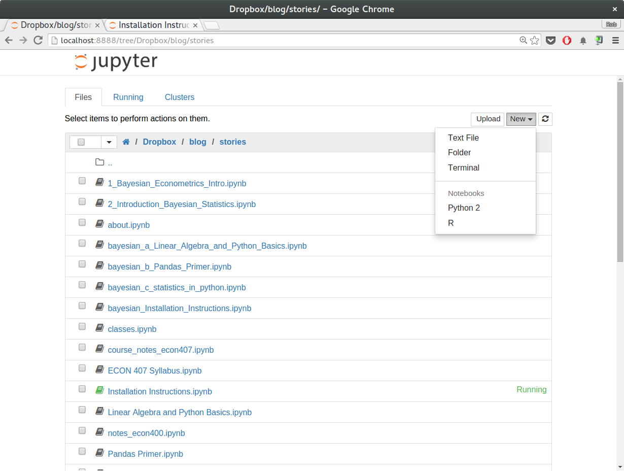\n",
"\n",
"You should see a terminal screen that looks something like this:\n",
"\n",
"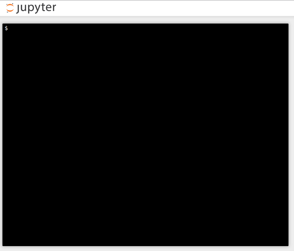\n",
"\n",
"In the terminal prompt, type\n",
"```\n",
"conda install seaborn\n",
"```\n",
"press enter and after a little time, it should install without incident.\n",
"\n",
"## Windows\n",
"\n",
"In Windows, choose Program Files -> Anaconda2 (64-bit) and you should see the following list of programs:\n",
"\n",
"\n",
"\n",
"Choose `Anaconda Prompt` and at the command prompt, type\n",
"```\n",
"conda install seaborn\n",
"```\n",
"press enter and after a little time, it should install without incident."
]
},
{
"cell_type": "markdown",
"metadata": {},
"source": [
""
]
},
{
"cell_type": "markdown",
"metadata": {},
"source": [
"# Installing pymc3 \n",
"\n",
"The best way to install packages is via the `conda` command. \n",
"\n",
"```\n",
"conda install pymc3\n",
"```\n",
"\n",
"The required compiler packages and other necessities should automatically be installed so that `pymc3` models will compile and run as required for this class."
]
}
],
"metadata": {
"hide_input": false,
"kernelspec": {
"display_name": "Python 3",
"language": "python",
"name": "python3"
},
"language_info": {
"codemirror_mode": {
"name": "ipython",
"version": 3
},
"file_extension": ".py",
"mimetype": "text/x-python",
"name": "python",
"nbconvert_exporter": "python",
"pygments_lexer": "ipython3",
"version": "3.9.12"
},
"latex_envs": {
"bibliofile": "biblio.bib",
"cite_by": "apalike",
"current_citInitial": 1,
"eqLabelWithNumbers": true,
"eqNumInitial": 0
}
},
"nbformat": 4,
"nbformat_minor": 2
}